Recurrent Neural Networks

What is a Recurrent Neural Network?

To solve the problem of sequences it comes recurrent neural network (RNN). Recurrent means happening repeatedly for certain time. In this case each time the model receives a new word from the sentence it will translate into English, this same step will be repeated for the rest of the words consequently the translation task will be recurrent. Moreover, it will remember the previous translated word and keep it in memory so when we translate the second one, we have the context.

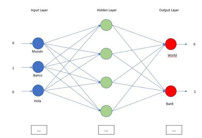
Feed forward neural network with input, hidden and output layers translating Spanish words to English — Feed forward neural network structure to translate incoming spanish words

Recurrent neural network unrolled over time steps translating a Spanish sentence word by word — Recurrent neural network structure to translate incoming spanish words

In the first image we see how a feed forward neural network will try to translate a full sentence. We create one-hot encoding for the sentence, this first layer will include all the possible Spanish words, if the word is present in the sentence like ‘banco’ we input 1 if not we input 0. The output layer is the same, a one-hot encoding for the English words. The major problem is the order is lost as we are providing a bag of words and not a sequence.

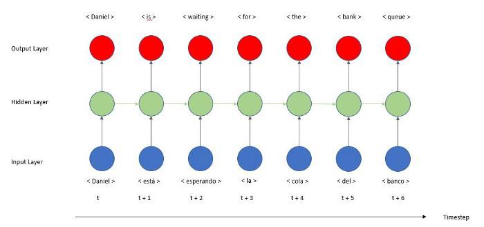
In the second image we see how a recurrent neural network will perform the same task. The first thing we notice is the model is no longer represented from left to right but instead from bottom to top. Why is that? We keep the x axes for the time step. A time step is the unit of action or time the model will do a task, in our case our time step is a word, so if we want to translate a sentence of 5 words we will have 5 time steps.

We still can see the first layer which is the input layer in blue that connects to a hidden layer in green. The second big difference we see compare to a FFNN where the cells in the hidden layer does not talk to each other, is that there is a new arrow from the cell of the previous step connecting with the next cell in the same layer. Here is the magic, in the second prediction the cell will not just receive the Spanish word but also will receive the context. The cell has created memory and now is using it to make the second prediction, instead of memory we refer to it as state. Finally, we see an output layer that will make the translation. From the prediction errors, we update the weights thanks to back propagation through time.

Need for a Neural Network dealing with Sequences

The beauty of recurrent neural networks lies in their diversity of application. When we are dealing with RNNs they have a great ability to deal with various input and output types.

Sentiment Classification

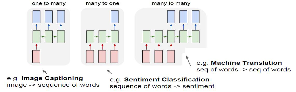
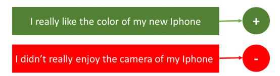
This can be a task of simply classifying tweets into positive and negative sentiment. So here the input would be a tweet of varying lengths, while output is of a fixed type and size.

Two example sentences classified as positive and negative sentiment

Image Captioning

Here, let’s say we have an image for which we need a textual description. So we have a single input – the image, and a series or sequence of words as output. Here the image might be of a fixed size, but the output is a description of varying lengths

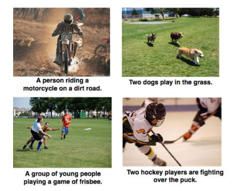
Four photos with generated captions: a person riding a motorcycle, two dogs playing in grass, people playing frisbee, hockey players

Language Translation

This basically means that we have some text in a particular language let’s say English, and we wish to translate it in French. Each language has it’s own semantics and would have varying lengths for the same sentence. So here the inputs as well as outputs are of varying lengths.

An English paragraph translated into French

Text Generations

Text generation output improving over training: from random characters to readable sentences after training more

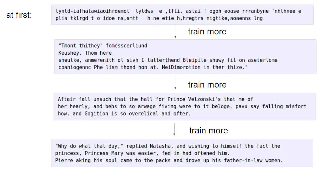
So RNNs can be used for mapping inputs to outputs of varying types, lengths and are fairly generalized in their application. Looking at their applications, let’s see how the architecture of an RNN looks like.

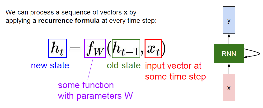
What are Recurrent Neural Networks?

We can process a sequence of vectors \(\mathbf{x}\) by applying a recurrence formula at every time step:

Recurrence formula h_t = f_W(h_{t-1}, x_t): new state from old state and input vector at some time step

Notice: the same function and the same set of parameters are used at every time step

The state consists of a single hidden vector h: h_t = tanh(W_hh h_{t-1} + W_xh x_t), y_t = W_hy h_t

An RNN with a feedback loop unfolded across time steps t-1, t, t+1 — Unfolding the recurrent loop across time steps

RNN computational graph, one to many: shared weights W feed f_W at every time step producing y_1 to y_T — RNN: Computational Graph: One to Many

Sequence to sequence: many-to-one encoder compressing the input into a single vector plus one-to-many decoder producing the output sequence — Sequence to Sequence: Many-to-one + one-to-many

Let me summarize the steps in a recurrent neuron for you

A single time step of the input is supplied to the network i.e. \(x_t\) is supplied to the network
We then calculate its current state using a combination of the current input and the previous state i.e. we calculate \(h_t\)
The current \(h_t\) becomes \(h_{t-1}\) for the next time step
We can go as many time steps as the problem demands and combine the information from all the previous states
Once all the time steps are completed the final current state is used to calculate the output \(y_t\)
The output is then compared to the actual output and the error is generated
The error is then backpropagated to the network to update the weights and the network is trained

Example

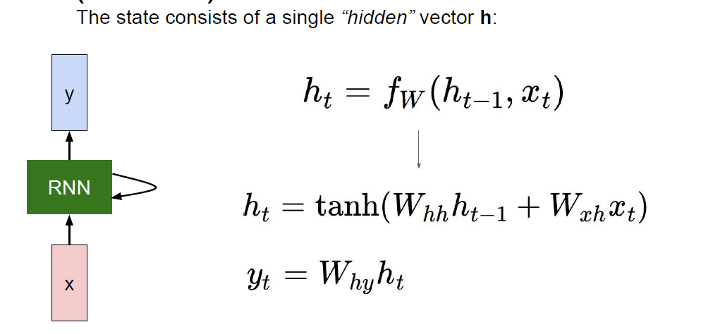
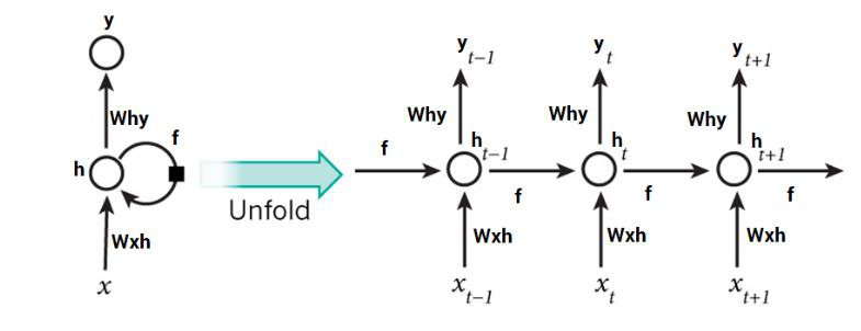
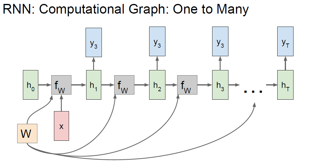
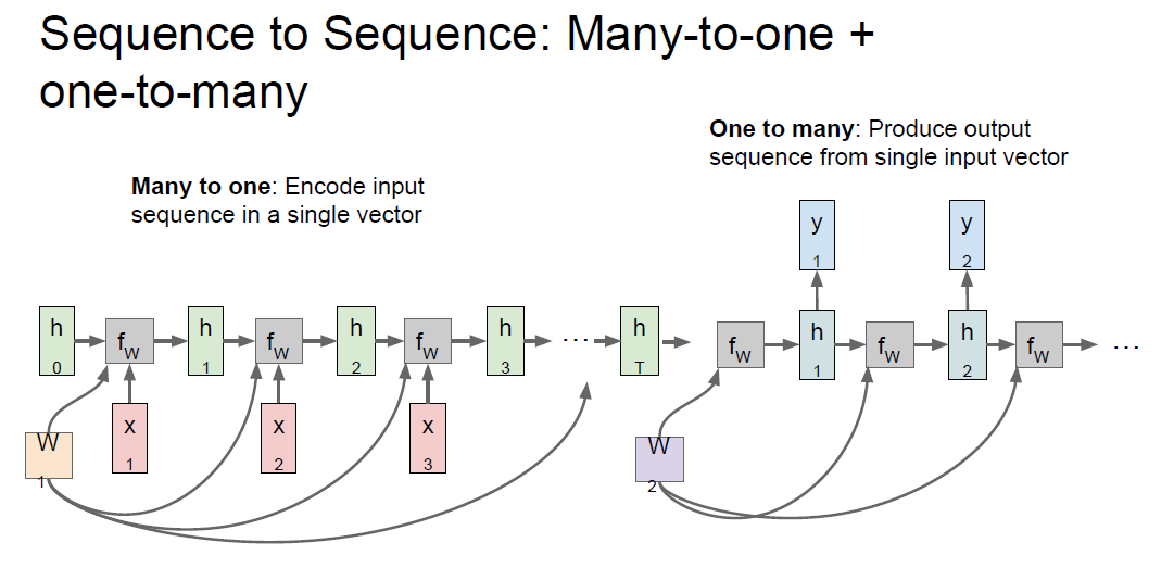
The state consists of a single “hidden” vector \(\mathbf{h}\):

\[ h_t = f_W(h_{t-1}, x_t) \]

\[ h_t = \tanh(W_{hh} h_{t-1} + W_{xh} x_t) \qquad y_t = W_{hy} h_t \]

Let’s take a look at the inputs first – the inputs are one hot encoded. Our entire vocabulary is {h,e,l,o} and hence we can easily one hot encode the inputs. Now the input neuron would transform the input to the hidden state using the weight \(w_{xh}\). We have randomly initialized the weights as a 3×4 matrix –

One hot encoded inputs for letters h, e, l, l over vocabulary {h,e,l,o}, and the randomly initialized 3x4 weight matrix wxh

Step 1: for the letter h, the hidden state needs Wxh times Xt; matrix multiplication gives the 3x1 result

Step 2: the recurrent neuron has Whh as a 1x1 weight matrix 0.427043 and bias 0.567001; for letter h the previous state is all zeros, so whh*ht-1+bias is computed

Step 3: current state h_t = tanh(Whh h_{t-1} + Wxh x_t); the two vectors are added and tanh is applied to get the current state

Step 4: the letter e is supplied; ht becomes ht-1 and the one hot encoded e is xt; Whh*ht-1+bias and Wxh*xt are computed

Step 5: ht for the letter e is computed by applying tanh to the sum

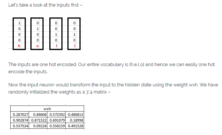
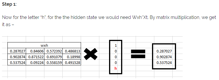
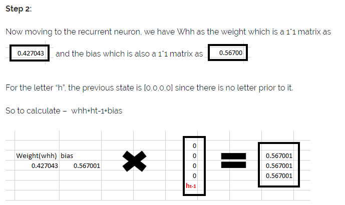
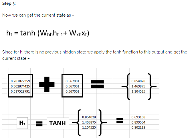
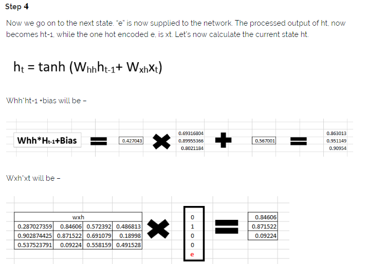
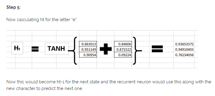
Now this would become \(h_{t-1}\) for the next state and the recurrent neuron would use this along with the new character to predict the next one.

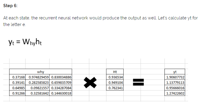
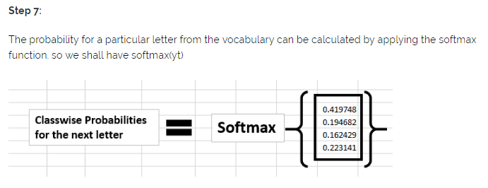
Step 6: at each state the RNN produces the output as well; yt = Why ht is calculated for the letter e

Step 7: softmax applied to yt gives classwise probabilities for the next letter

If we convert these probabilities to understand the prediction, we see that the model says that the letter after “e” should be h, since the highest probability is for the letter “h”. Does this mean we have done something wrong? No, so here we have hardly trained the network. We have just shown it two letters. So it pretty much hasn’t learnt anything yet.

Now the next BIG question that faces us is how does Back propagation work in case of a Recurrent Neural Network. How are the weights updated while there is a feedback loop?

Problems with RNN

Exploding and vanishing gradient problems during backpropagation.

Gradients are those values which to update neural networks weights. In other words, we can say that Gradient carries information.

Vanishing gradient is a big problem in deep neural networks. it vanishes or explodes quickly in earlier layers and this makes RNN unable to hold information of longer sequence. and thus RNN becomes short-term memory.

If we apply RNN for a paragraph RNN may leave out necessary information due to gradient problems and not be able to carry information from the initial time step to later time steps.

To solve this problem LSTM, GRU came into the picture.

How do LSTM, GRU solve this problem?

I highly encourage you to read Colah’s blog for in-depth knowledge of LSTM.

The reason for exploding gradient was the capturing of relevant and irrelevant information. a model which can decide what information from a paragraph and relevant and remember only relevant information and throw all the irrelevant information

This is achieved by using gates. the LSTM ( Long -short-term memory ) and GRU ( Gated Recurrent Unit ) have gates as an internal mechanism, which control what information to keep and what information to throw out. By doing this LSTM, GRU networks solve the exploding and vanishing gradient problem.

Almost each and every SOTA ( state of the art) model based on RNN follows LSTM or GRU networks for prediction.

LSTMs /GRUs are implemented in speech recognition, text generation, caption generation, etc.

LSTM networks

Every LSTM network basically contains three gates to control the flow of information and cells to hold information. The Cell States carries the information from initial to later time steps without getting vanished.

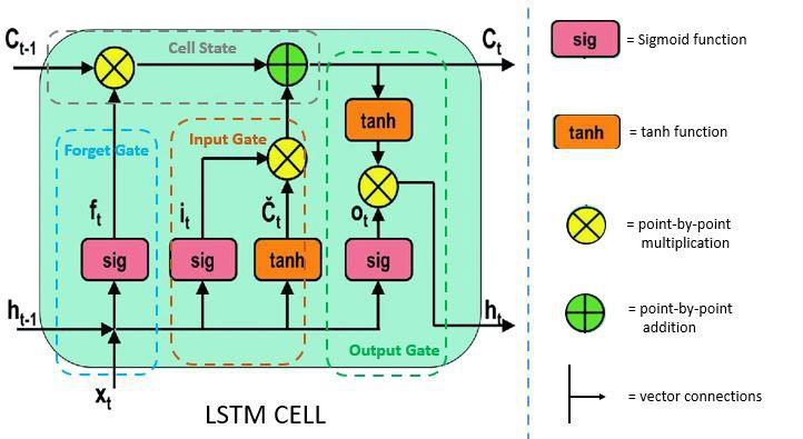
LSTM cell diagram showing the cell state, forget gate, input gate and output gate with sigmoid and tanh functions — LSTM CELL

Gates

Gates make use of sigmoid activation or you can say tanh activation. values ranges in tanh activation are 0 -1.

1

Forget Gate

This gate decides what information should be carried out forward or what information should be ignored.

Information from previous hidden states and the current state information passes through the sigmoid function. Values that come out from sigmoid are always between 0 and 1. if the value is closer to 1 means information should proceed forward and if value closer to 0 means information should be ignored.

2

Input Gate

After deciding the relevant information, the information goes to the input gate, Input gate passes the relevant information, and this leads to updating the cell states. simply saving updating the weight.

Input gate adds the new relevant information to the existing information by updating cell states.

3

Output Gate

After the information is passed through the input gate, now the output gate comes into play. Output gate generates the next hidden states. and cell states are carried over the next time step.

GRU

Gated Recurrent Network (GRU) cell diagram with update gate and reset gate — Gated Recurrent Network (GRU)

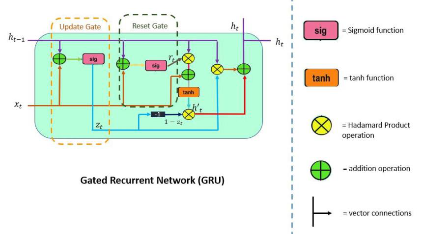
GRU ( Gated Recurrent Units ) are similar to the LSTM networks. GRU is a kind of newer version of RNN. However, there are some differences between GRU and LSTM.

GRU doesn’t contain a cell state
GRU uses its hidden states to transport information
It Contains only 2 gates(Reset and Update Gate)
GRU is faster than LSTM
GRU has lesser tensor’s operation that makes it faster

1

Update Gate

Update Gate is a combination of Forget Gate and Input Gate. Forget gate decides what information to ignore and what information to add in memory.

2

Reset Gate

This Gate Resets the past information in order to get rid of gradient explosion. Reset Gate determines how much past information should be forgotten.

BI-LSTM Networks

Bidirectional LSTM with a forward layer and a backward layer of LSTM cells feeding an activation layer and outputs

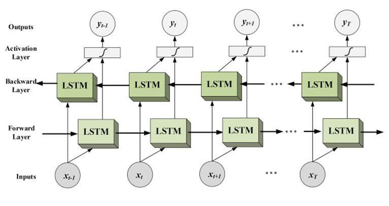
We have seen how LSTM works and we noticed that it works in uni-direction.

Bidirectional long-short term memory networks are advancements of unidirectional LSTM. Bi-LSTM tries to capture information from both sides left to right and right to left. The rest of the concept in Bi-LSTM is the same as LSTM.

This improves the accuracy of models.

Interactive: LSTM · GRU · Bi-LSTM Simulator

See the gates compute with real numbers — step through every σ and tanh, drag the forget bias to watch long-term memory appear and vanish, and follow a Bi-LSTM's forward and backward passes cell by cell.

Open the Simulator

Practice in PyTorch: TorchCode

Implement an RNN cell's forward pass — the same \(h_t = \tanh(W_{hh}h_{t-1} + W_{xh}x_t)\) recurrence worked by hand above — and check it against PyTorch: instant feedback, reference solutions, no GPU needed.

Open TorchCode