Deep Feedforward Networks Tutorial

Introduction to Deep Feedforward Networks

Understanding the quintessential deep learning models

What are Deep Feedforward Networks?

Deep feedforward networks, also called feedforward neural networks or multilayer perceptrons (MLPs), are the quintessential deep learning models. The goal of a feedforward network is to approximate some function f*.

For example, for a classifier, y = f*(x) maps an input x to a category y. A feedforward network defines a mapping y = f(x; θ) and learns the value of the parameters θ that result in the best function approximation.

Why "Feedforward"?

These models are called feedforward because information flows through the function being evaluated from x, through the intermediate computations used to define f, and finally to the output y.

Feedforward Networks

No feedback connections - information flows in one direction

Recurrent Networks

Include feedback connections where outputs are fed back into the model

Importance in Machine Learning

Commercial Applications

Form the basis of many important commercial applications

Computer Vision

Convolutional networks for object recognition are specialized feedforward networks

Foundation

Conceptual stepping stone to recurrent networks for NLP

Key Concepts

Understanding the fundamental building blocks

Network Structure

Feedforward neural networks are called networks because they are typically represented by composing together many different functions. The model is associated with a directed acyclic graph describing how the functions are composed together.


# Example: Three functions connected in a chain
f(x) = f³(f²(f¹(x)))

# Where:
# f¹ is the first layer
# f² is the second layer  
# f³ is the third layer (output layer)

The overall length of the chain gives the depth of the model. The name "deep learning" arose from this terminology.

Hidden Layers

The training data provides us with noisy, approximate examples of f*(x) evaluated at different training points. Each example x is accompanied by a label y ≈ f*(x).

Output Layer

Training examples specify directly what the output layer must do at each point x

Hidden Layers

Training data does not show the desired output for these layers - they are "hidden"

The learning algorithm must decide how to use hidden layers to best implement an approximation of f*.

Neural Inspiration

These networks are called neural because they are loosely inspired by neuroscience. Each hidden layer of the network is typically vector valued, and each element may be interpreted as playing a role analogous to a neuron.

Biological Neuron

Receives input from many other neurons
Computes its own activation value
Sends output to other neurons

Artificial Neuron

Receives input from many other units
Computes its own activation value
Represents vector-to-scalar function

Modern neural networks are best thought of as function approximation machines designed to achieve statistical generalization, rather than as models of brain function.

Overcoming Limitations of Linear Models

Why we need nonlinear transformations

Limitations of Linear Models

Linear models, such as logistic regression and linear regression, are appealing because they can be fit efficiently and reliably, either in closed form or with convex optimization.

Advantages

Efficient and reliable fitting
Closed form solutions
Convex optimization

Limitations

Limited to linear functions
Cannot understand interaction between input variables
Poor capacity for complex patterns

Extending Linear Models

To extend linear models to represent nonlinear functions of x, we can apply the linear model not to x itself but to a transformed input φ(x), where φ is a nonlinear transformation.


# Instead of: y = w^T x + b
# We use:     y = w^T φ(x) + b

# Where φ(x) is a nonlinear transformation that:
# - Provides a set of features describing x
# - Provides a new representation for x

The key question: How do we choose the mapping φ?

Approaches to Feature Mapping

Three strategies for choosing φ(x)

1. Generic φ

Use a very generic φ, such as the infinite-dimensional φ that is implicitly used by kernel machines based on the RBF kernel.

Pros:

High dimensional capacity
Can fit training set

Cons:

Poor generalization to test set
Based only on local smoothness
Doesn't encode enough prior information

2. Manual Engineering

Manually engineer φ. Until the advent of deep learning, this was the dominant approach.

Pros:

Domain expertise incorporated
Proven in specific domains

Cons:

Requires decades of human effort
Domain-specific specialization
Little transfer between domains

3. Deep Learning

Learn φ. We have a model y = f(x; θ, w) = φ(x; θ)ᵀw with parameters θ to learn φ and parameters w to map to output.

Pros:

Highly generic when needed
Can incorporate human knowledge
Only need to find right function family
Benefits outweigh harms

Cons:

Gives up convexity of training problem

The Winner: Deep Learning Strategy

The deep learning approach is the only one that gives up on the convexity of the training problem, but the benefits outweigh the harms. This approach parametrizes the representation as φ(x; θ) and uses optimization algorithms to find the θ that corresponds to a good representation.

Key Insight: The human designer only needs to find the right general function family rather than finding precisely the right function.

Example: Learning XOR

A concrete example of feedforward networks in action

The XOR Problem

The XOR function ("exclusive or") is an operation on two binary values, x₁ and x₂. When exactly one of these binary values is equal to 1, the XOR function returns 1. Otherwise, it returns 0.

XOR Truth Table

x₁	x₂	XOR Output
0	0	0
0	1	1
1	0	1
1	1	0

Goal: Train a network to perform correctly on all four points: X = {[0,0], [0,1], [1,0], [1,1]}

Why Linear Models Fail

Suppose we choose a linear model with θ consisting of w and b. Our model is defined as:


f(x; w, b) = x^T w + b

# Using mean squared error loss function:
J(θ) = (1/4) Σ (f*(x) - f(x; θ))²

After solving the normal equations, we obtain w = 0 and b = 1/2. The linear model simply outputs 0.5 everywhere!

Why This Happens:

When x₁ = 0, the model's output must increase as x₂ increases
When x₁ = 1, the model's output must decrease as x₂ increases
A linear model must apply a fixed coefficient w₂ to x₂
The linear model cannot use the value of x₁ to change the coefficient on x₂

Solution: Feedforward Network

We introduce a simple feedforward network with one hidden layer containing two hidden units.


# Network structure:
h = f¹(x; W, c)    # Hidden layer
y = f²(h; w, b)    # Output layer

# Complete model:
f(x; W, c, w, b) = f²(f¹(x))

# Hidden layer computation:
h = g(W^T x + c)   # where g is activation function

Key Insight: If f¹ were linear, the entire network would remain linear. We must use a nonlinear activation function g.

Activation Functions

Most neural networks use an affine transformation controlled by learned parameters, followed by a fixed nonlinear function called an activation function.

Rectified Linear Unit (ReLU)


g(z) = max{0, z}

# Properties:
# - Default recommendation
# - Piecewise linear function
# - Preserves linear model properties
# - Easy to optimize
# - Good generalization

ReLU Function

Universal Function Approximation: We can build a universal function approximator from rectified linear functions, much like a Turing machine can be built from minimal components.

Visualizing the XOR Solution

How neural networks transform the problem space

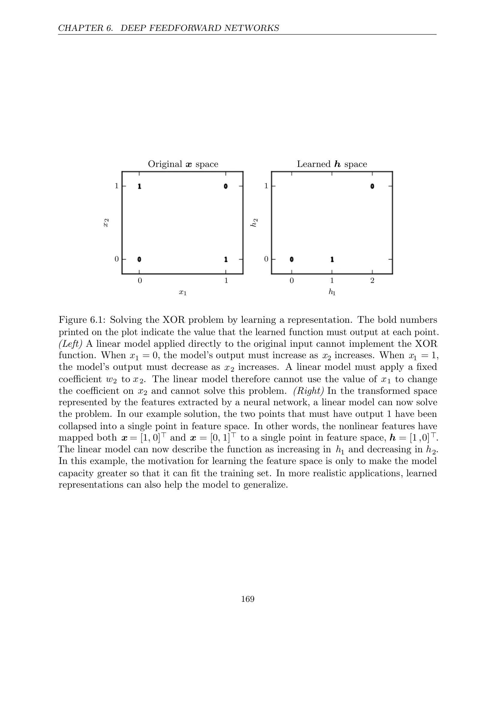
Figure 6.1: Learning a Representation

Key Insights:

Left: Linear model cannot implement XOR in original space
Right: In transformed space, linear model can solve the problem
Points [1,0] and [0,1] are mapped to the same point [1,0] in feature space
Linear model can now increase in h₁ and decrease in h₂

The nonlinear features have mapped both x = [1,0] and x = [0,1] to a single point in feature space, h = [1,0]. This transformation makes the problem linearly separable.

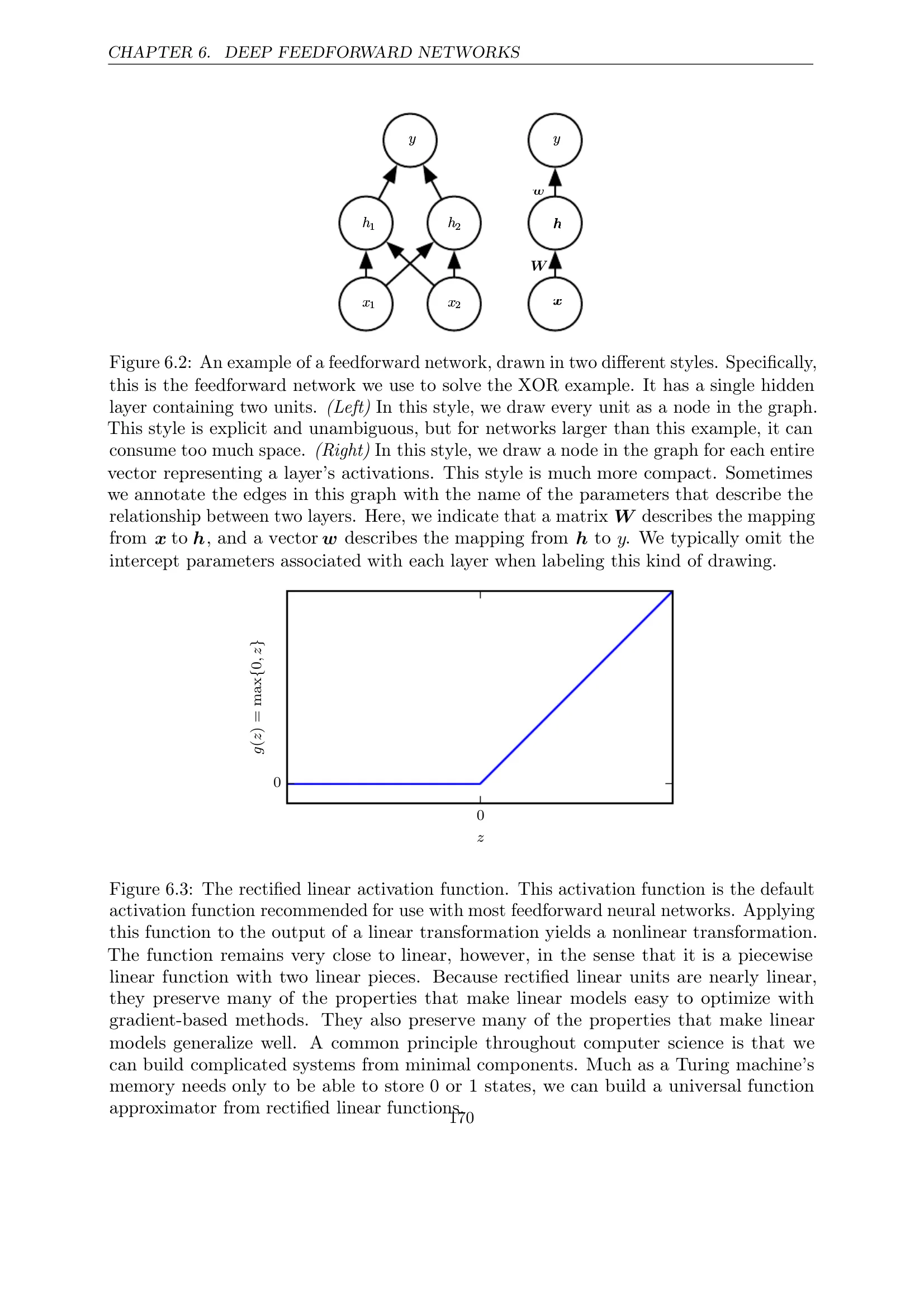
Figure 6.2: Network Architecture

Two Drawing Styles:

Left: Every unit as a node - explicit but space-consuming
Right: Vector representation - more compact
Matrix W describes mapping from x to h
Vector w describes mapping from h to y

Figure 6.3: ReLU Activation Function

ReLU Properties:

Default choice for most feedforward networks
Piecewise linear with two linear pieces
Nearly linear - preserves optimization properties
Good generalization properties
Universal approximation capability

Interactive ReLU Function

Move your mouse over the graph to see values

Key Takeaways

Essential insights from deep feedforward networks

Nonlinearity is Essential

Linear transformations alone cannot solve complex problems like XOR. Nonlinear activation functions are crucial for learning complex patterns.

Feature Learning

Deep learning automatically learns useful representations, eliminating the need for manual feature engineering in most cases.

Layer Composition

Multiple layers allow complex function approximation through composition of simpler functions, enabling deep networks to model intricate patterns.

Hidden Layers

Intermediate representations are not directly specified by training data, allowing the network to learn optimal internal representations.

Conclusion

Deep feedforward networks overcome the limitations of linear models through learned feature representations and nonlinear transformations. They provide the foundation for understanding more complex deep learning models and have revolutionized machine learning across numerous domains.

Review Tutorial Download Notes