Introduction to Machine Learning

What You'll Learn

How AI, Machine Learning and Deep Learning relate to each other
Tom Mitchell's definition of learning: Task, Performance, Experience (T–P–E)
The four components of learning and where ML is used today
The learning types: supervised, unsupervised, semi-supervised and reinforcement learning
The three model families: logical, geometric and probabilistic
A first look at evaluation: under/overfitting, the bias–variance trade-off, train/validation/test splits and cross-validation

Tools for this course: Python in Google Colab (free, nothing to install) or a local IDE such as PyCharm, with numpy, pandas, matplotlib and scikit-learn.

1. AI, Machine Learning and Deep Learning

Artificial Intelligence (AI) is the science of building systems that simulate and extend human intelligence. John McCarthy coined the term in 1956 and defined it as “the science and engineering of making intelligent machines, especially intelligent computer programs”.

Machine Learning (ML) is the part of AI that studies how computers can acquire knowledge or skills from data and improve their performance with experience, instead of being explicitly programmed with rules. An intelligent system that cannot learn is hard to call intelligent at all.

Deep Learning (DL) is the part of ML built on artificial neural networks with many hidden layers. It is the engine behind modern image, sound and text understanding.

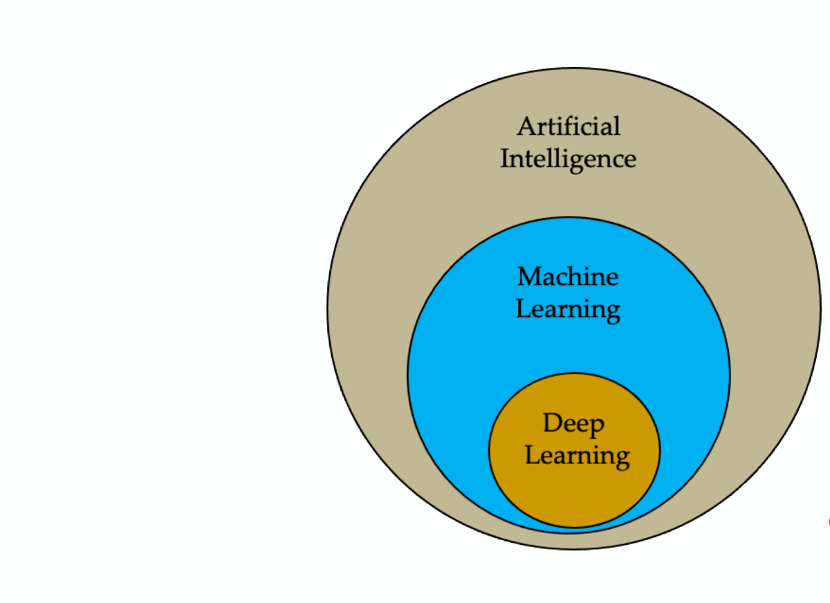
Nested circles: Deep Learning inside Machine Learning inside Artificial Intelligence — Deep learning ⊂ machine learning ⊂ artificial intelligence. Every ML system needs four elements: **data, an algorithm, computing power, and a scenario** (a problem worth solving). *(From Dr. Albanna's slides.)*

Rules vs. learning

A traditional program takes rules + data → answers. A machine-learning program takes data + answers → rules (a model). The model is then applied to new data it has never seen.

2. What Does It Mean to Learn? (T–P–E)

Learning, for people, is “the activity or process of gaining knowledge or skill by studying, practicing, being taught, or experiencing something” (Merriam-Webster). For machines we use Tom Mitchell's precise definition:

A program learns from experience E with respect to tasks T and performance measure P,
if its performance at T, as measured by P, improves with E.

Data (experience) enters a learning algorithm (task) to produce understanding (performance) — Data is the experience, the learning algorithm performs the task, and the result is judged by a performance measure. *(From Dr. Albanna's slides.)*

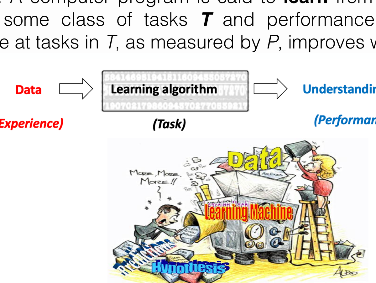
Problem	Task T	Performance P	Experience E
Handwriting recognition	Recognize and classify handwritten words in images	% of words correctly classified	A database of labelled handwritten words
Robot driving	Drive on public highways using vision sensors	Average distance travelled before an error	Images and steering commands recorded from a human driver
Chess	Play chess	% of games won against opponents	Games played against itself
Spam filtering	Label e-mails as spam / not spam	% of e-mails correctly labelled	E-mails the user has marked as spam

3. The Components of Learning

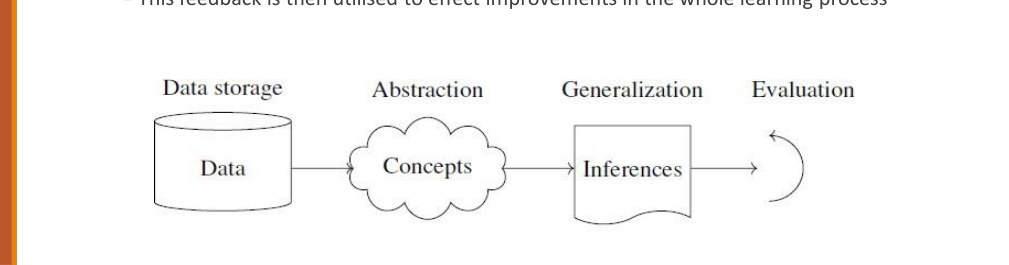
Whether the learner is a human or a machine, the process breaks into four parts:

Data storage — keeping and retrieving large amounts of data; the foundation for reasoning.
Abstraction — extracting knowledge from the stored data by building concepts and models that summarize it.
Generalization — turning that knowledge into a form that works on future data that is similar to, but not the same as, what was seen. This is the real goal of ML.
Evaluation — measuring how useful the learned knowledge is, and feeding the result back to improve the whole process.

Data storage, abstraction, generalization, evaluation — Data → concepts → inferences → evaluation. *(University course slides; the four components follow B. Lantz, *Machine Learning with R*, Packt.)*

4. AI Is Everywhere: Applications

“The last 10 years have been about building a world that is mobile-first. In the next 10 years we will shift to a world that is AI-first” — Sundar Pichai. You already use ML every day:

Area	Examples
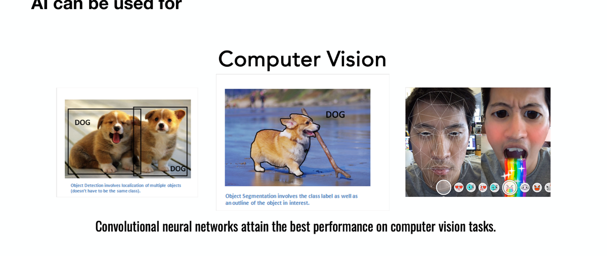
Computer vision	Face recognition, object detection, medical imaging (retina scans), self-driving cars
Speech & language	Speech-to-text, voice assistants, Google Translate, sentiment analysis, spam filtering
Recommendation	Netflix, Amazon and YouTube suggestions; Instagram feed ranking
Finance & business	Credit scoring, fraud detection, customer segmentation, algorithmic trading
Games & robotics	AlphaGo, Atari-playing agents, robot control
Generative AI	GANs and diffusion models that create realistic images; large language models

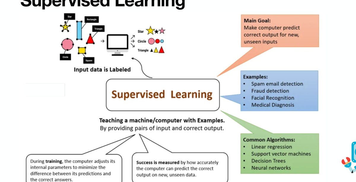
Computer vision examples: image classification and face filters — Convolutional neural networks reach the best performance on computer-vision tasks. *(From Dr. Albanna's slides.)*

5. Supervised Learning

In supervised learning every training example comes with the correct answer (a label). The algorithm learns a function that maps inputs to outputs, then predicts the label of new, unseen inputs. It is a predictive task: like a student learning from solved examples.

A robot is shown labelled pictures of cats, dogs and bunnies, then names a new picture — We help the machine learn by labelling each picture. Shown a new picture, it answers “It's a dog”. *(From Dr. Albanna's slides.)*

Two kinds of supervised problem

	Classification	Regression
Output	A category (class)	A continuous number
Question	“Which class?”	“How much?”
Examples	Spam / not spam; cat / dog; admit / reject a student; disease / healthy	House price from size; exam score from study hours; temperature tomorrow
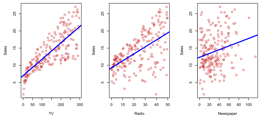
Algorithms in this course	Logistic regression, decision trees, Naïve Bayes, SVM, neural networks	Linear regression (Module 3)

Supervised learning summary: goal, examples, common algorithms — Supervised learning at a glance: the goal, real uses (spam detection, fraud detection, face recognition, medical diagnosis) and the common algorithms. *(From Dr. Albanna's slides.)*

Sales plotted against TV, radio and newspaper advertising budgets, each with a fitted line — A real regression problem: predict **sales** (the output) from the advertising budgets for TV, radio and newspaper (the inputs) in 200 markets. Each blue line is a simple least-squares fit — exactly what Module 3 teaches. *(Textbook T1: James, Witten, Hastie & Tibshirani, An Introduction to Statistical Learning with Applications in Python, Springer 2023, Figure 2.1.)*

Worked example — spam filtering

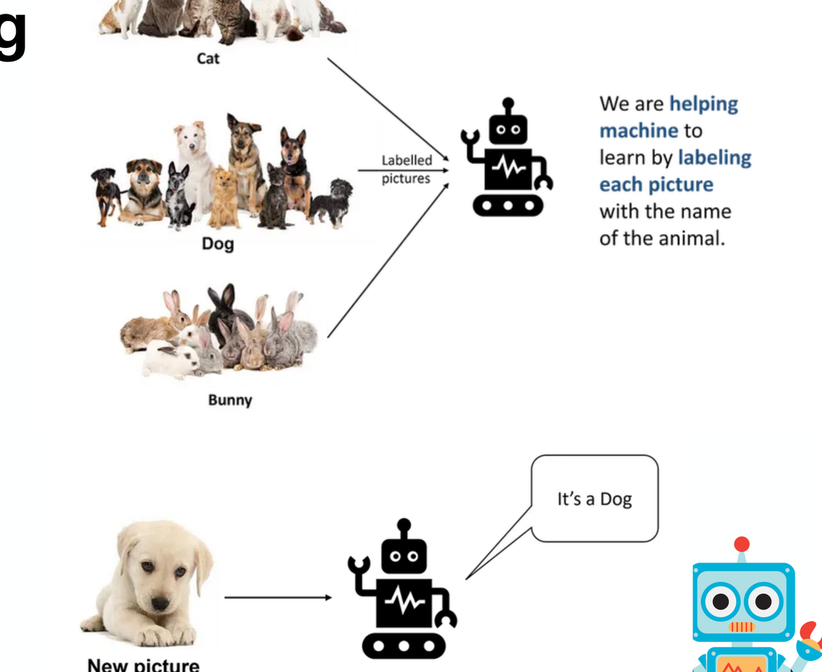
100 e-mails were flagged by hand: 25 spam and 75 not spam. These 100 labelled e-mails are the training set. A classifier learns which words and senders separate the two groups, and then labels each new e-mail on arrival. Because the output is one of two categories, this is binary classification.

6. Unsupervised Learning

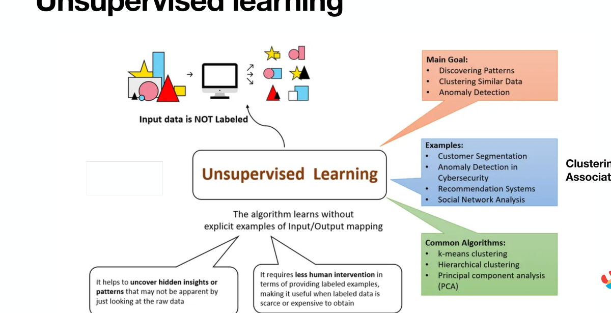
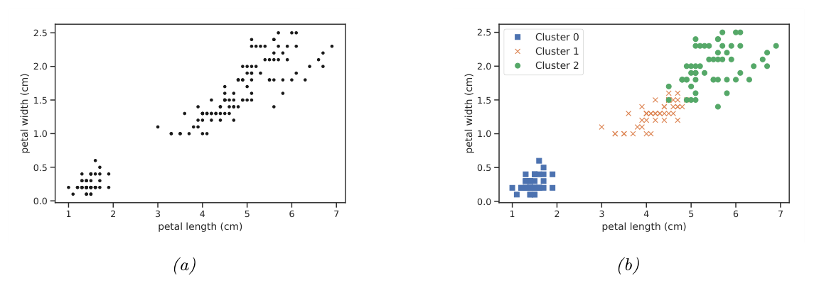
In unsupervised learning the data has no labels. The algorithm looks for structure on its own — groups of similar items, unusual items, or items that occur together. It is a descriptive task: there is no correct answer to compare against.

Unsupervised learning summary: goal, examples, common algorithms — Unsupervised learning at a glance. *(From Dr. Albanna's slides.)*

Iris petal measurements without labels, then grouped into three clusters by k-means — (a) The iris flowers with their labels removed: just petal length and width. (b) k-means (K = 3) discovers three groups on its own, with no answers given. Compare with the labelled iris data used in the Python lab below. *(Textbook T2: K. P. Murphy, Probabilistic Machine Learning: An Introduction, MIT Press 2022, Figure 1.8; CC BY-NC-ND.)*

Clustering — customer segmentation: group shoppers with similar purchasing behaviour for targeted marketing (k-means, Module 10).
Anomaly detection — flag unusual network traffic as a possible security threat.
Association — “customers who bought X also bought Y”.
Recommendation — suggest products, movies or content from patterns in user behaviour.
Dimensionality reduction — compress many features into a few (e.g. PCA, Module 2).

7. Semi-supervised Learning

Labelling is slow and expensive; unlabelled data is cheap. Semi-supervised learning uses a small labelled set plus a large unlabelled set. For example, to recommend web pages we would need users to mark pages they like — few will do it, but we have millions of unlabelled pages. The algorithm learns from the few labels and uses the structure of the unlabelled data to improve.

8. Reinforcement Learning

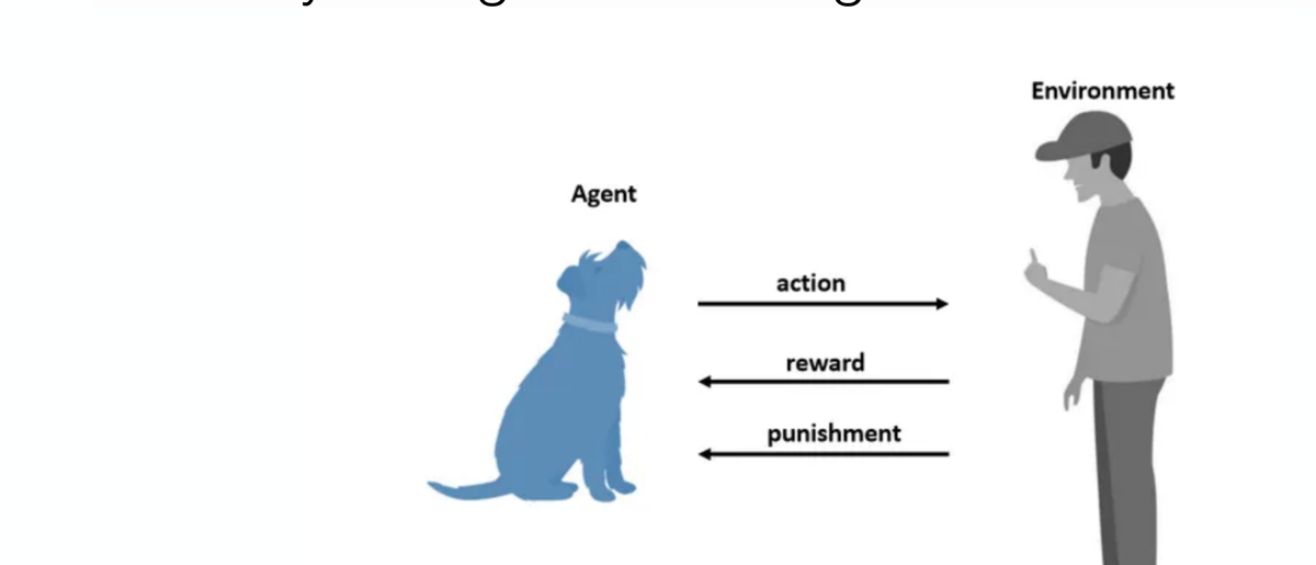
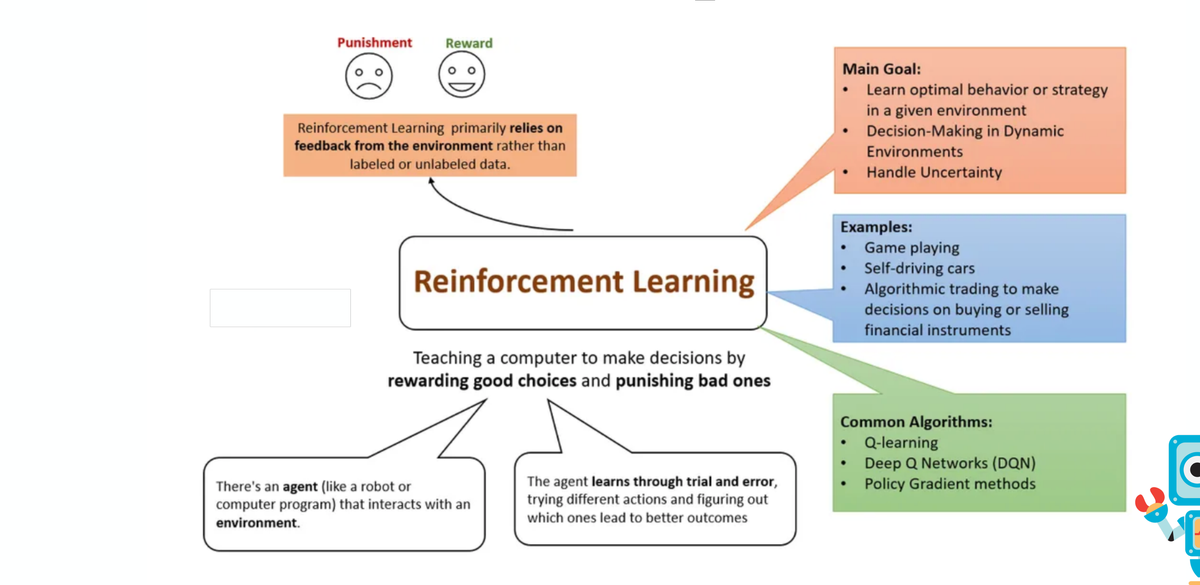
In reinforcement learning (RL) an agent learns by trial and error. It takes an action in an environment, receives a reward or punishment, and adjusts its behaviour to maximize the total reward over time — just as you train a dog with treats.

Agent (dog) acts; environment (trainer) returns reward or punishment — The agent acts; the environment answers with a reward or a punishment. *(From Dr. Albanna's slides.)*

Reinforcement learning summary: goal, examples, common algorithms — Reinforcement learning at a glance: game playing, self-driving cars, algorithmic trading; Q-learning and Deep Q-Networks. *(From Dr. Albanna's slides.)*

AlphaGo (DeepMind) learned to play Go at superhuman level and defeated the world champions.
Self-driving cars learn to navigate traffic and make decisions at intersections.
Algorithmic trading agents learn when to buy and sell from market data.

	Supervised	Unsupervised	Reinforcement
Data	Labelled examples	Unlabelled examples	No dataset; interaction with an environment
Feedback	The correct answer	None	A delayed reward signal
Goal	Predict labels	Discover structure	Learn a policy that maximizes reward

9. Three Families of Models

Every algorithm in this course builds a model — a summary of the data that lets us make predictions. Models fall into three families by how they describe the data:

Family	Idea	Examples in this course
Logical	Divide the instance space with logical expressions (IF–THEN rules)	Decision trees (Module 6), rule sets
Geometric	Treat examples as points in space; use lines, planes and distances	Linear regression, SVM, k-nearest neighbours, k-means
Probabilistic	Treat features and targets as random variables; model the uncertainty with probabilities	Naïve Bayes (Module 7), logistic regression

Probabilistic models are either discriminative (model P(Y|X) directly) or generative (model the joint P(Y, X) and use Bayes' rule):

\[ P(A \mid B) = \frac{P(B \mid A)\,P(A)}{P(B)} \]

10. Generalization: Underfitting, Overfitting, Bias and Variance

A model is only useful if it works on new data. Two things can go wrong:

	Underfitting	Overfitting
What happens	Model is too simple to capture the pattern	Model memorizes noise in the training data
Training accuracy	Low	Very high
Test accuracy	Low	Low
Error type	High bias	High variance
Typical fix	More features, a more flexible model, train longer	More data, a simpler model, regularization, pruning

Bias is how far the model's predictions are, on average, from the truth. High bias means strong simplifying assumptions and underfitting.
Variance is how much the predictions change when we train on a different sample of data. High variance means overfitting.

Four targets: low/high bias crossed with low/high variance — Bias is the distance from the bull's-eye; variance is the spread of the shots. We want low bias *and* low variance. *(University course slides; diagram after S. Fortmann-Roe, “Understanding the Bias–Variance Tradeoff”, 2012.)*

Bias falls and variance rises as model complexity grows; total error is U-shaped — As model complexity grows, bias² falls and variance rises. Total error is U-shaped; the best model sits at the bottom of the U. *(University course slides.)*

Left: three fits of increasing flexibility. Right: training error keeps falling while test error is U-shaped — **Left:** the true function (black) and three fits: a straight line (orange, underfits), a moderate curve (blue, about right) and a very wiggly curve (green, overfits). **Right:** as flexibility grows, the training error keeps falling but the test error falls and then rises. The dashed line is the irreducible error. *(Textbook T1: James, Witten, Hastie & Tibshirani, An Introduction to Statistical Learning with Applications in Python, Springer 2023, Figure 2.9.)*

Polynomials of degree 2, 14 and 20 fit to 21 points, and train/test MSE against degree — The same lesson with polynomials fit to 21 points: degree 2 is smooth, degree 14 starts chasing the noise, and degree 20 passes through every point but swings wildly between them. In (d), training error keeps dropping with the degree while test error climbs — overfitting. *(Textbook T2: K. P. Murphy, Probabilistic Machine Learning: An Introduction, MIT Press 2022, Figure 1.7; CC BY-NC-ND.)*

11. A First Look at Evaluation

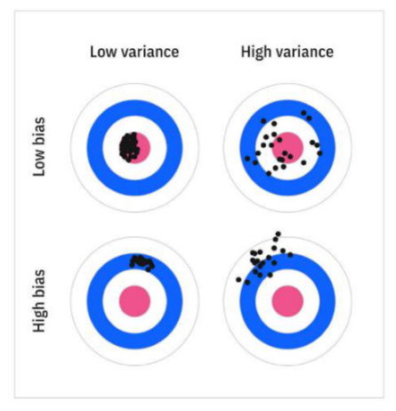
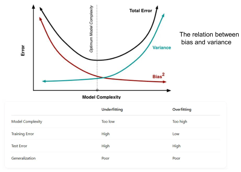
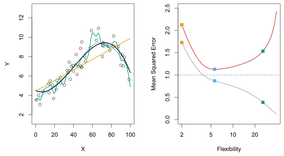
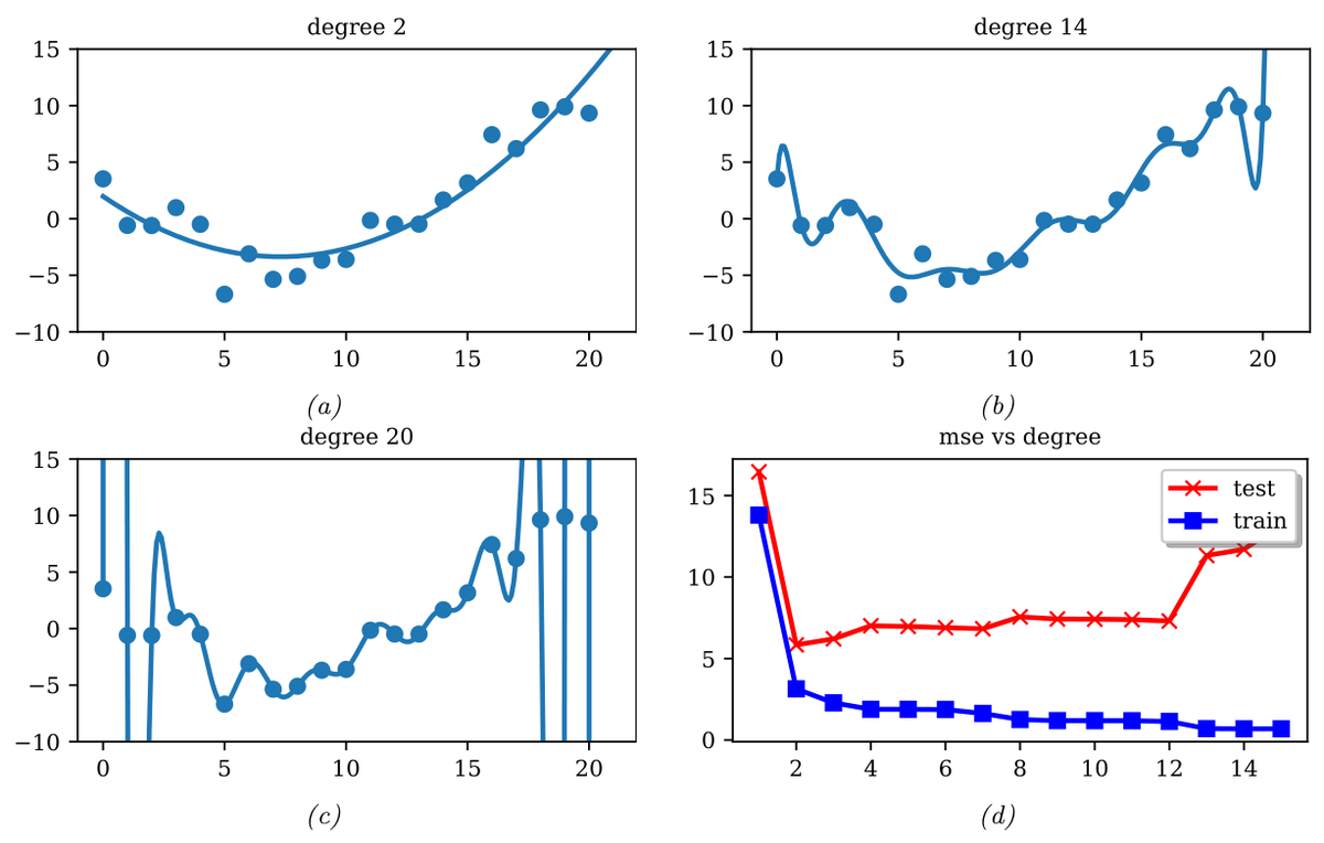
To estimate how a model will do on unseen data, we must test it on data it did not train on. The usual split:

Training set (~50–70%) — used to fit the model's parameters.
Validation set (~15–25%) — used to choose hyperparameters (settings we pick, such as tree depth, learning rate, or number of clusters).
Test set (~15–25%) — touched once at the end to report the final performance.

k-fold cross-validation

When data is scarce, split it into k equal folds. Train on k−1 folds and validate on the remaining one; repeat k times so every fold is used once for validation, then average the k scores.

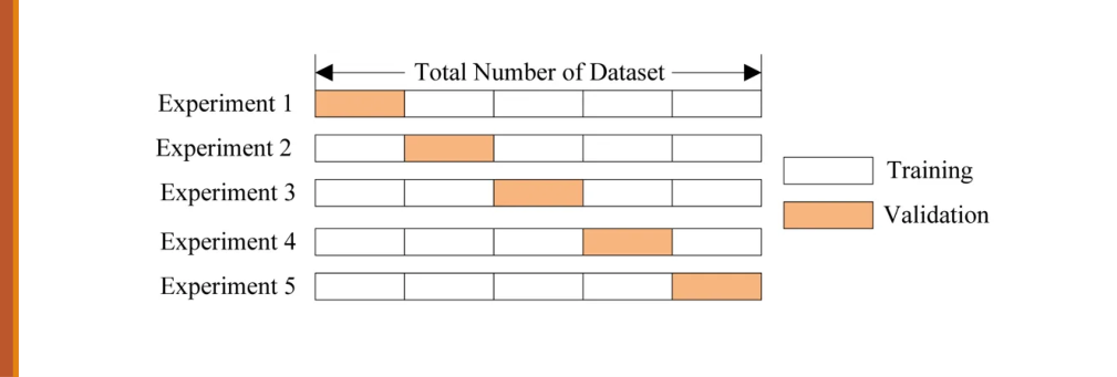
Five experiments, each using a different fold for validation — 5-fold cross-validation: each experiment holds out a different fold. *(University course slides.)*

Worked example

A dataset has 1,000 rows. A 50/25/25 split gives 500 training, 250 validation and 250 test rows. With 5-fold cross-validation on the 750 non-test rows, each fold has 750 / 5 = 150 rows: every model trains on 600 rows and validates on 150. If the five validation accuracies are 0.82, 0.85, 0.80, 0.84 and 0.84, the cross-validated accuracy is (0.82+0.85+0.80+0.84+0.84) / 5 = 0.83.

Module 5 covers the measures themselves (accuracy, precision, recall, F1, ROC/AUC, MAE, RMSE, R²).

Your First Model in Python

Open a new notebook in Google Colab and run this. It follows the full workflow from this module: load labelled data, split it, train a classifier, and evaluate it on unseen data.

from sklearn.datasets import load_iris
from sklearn.model_selection import train_test_split, cross_val_score
from sklearn.tree import DecisionTreeClassifier

X, y = load_iris(return_X_y=True)          # 150 flowers, 4 features, 3 classes (labelled = supervised)
X_train, X_test, y_train, y_test = train_test_split(
    X, y, test_size=0.25, random_state=42, stratify=y)

model = DecisionTreeClassifier(max_depth=3)   # max_depth is a hyperparameter
model.fit(X_train, y_train)                       # learn from experience E
print("Train accuracy:", model.score(X_train, y_train))
print("Test accuracy :", model.score(X_test, y_test))   # performance P on unseen data

scores = cross_val_score(DecisionTreeClassifier(max_depth=3), X, y, cv=5)
print("5-fold CV accuracy:", scores.mean().round(3))

Try it

Change max_depth to 1 and then to 20. Which setting underfits (both accuracies low)? Which one makes the training accuracy perfect while the test accuracy stops improving?

Textbook Reading

From the course syllabus

T1 James, Witten, Hastie & Tibshirani — An Introduction to Statistical Learning with Applications in Python, Ch. 1 (and §2.1–2.2 on the bias–variance trade-off).
T2 Murphy — Probabilistic Machine Learning: An Introduction, Ch. 1 (§1.2 supervised learning, §1.3 unsupervised learning).

Both books are free to read online from their authors: statlearning.com (T1) and probml.github.io (T2).

Exercises

1

Define T, P and E

A bank wants a system that predicts whether a loan applicant will default. Write the task T, performance measure P and experience E.

T: classify each applicant as “will default” or “will repay”. P: % of applicants classified correctly (or better, recall on the defaulters, since missing a defaulter is costly). E: historical loan records of past applicants, each labelled with whether they defaulted.

2

Which type of learning?

Name the learning type for each: (a) grouping news articles by topic with no topic labels; (b) predicting tomorrow's temperature from past weather records; (c) teaching a robot to walk by rewarding forward progress; (d) detecting fraudulent card transactions from transactions already marked fraud / legitimate.

(a) Unsupervised (clustering). (b) Supervised — regression (numeric output). (c) Reinforcement learning. (d) Supervised — classification (fraud / legitimate).

3

Classification or regression?

(a) a student's final mark out of 100; (b) whether a student passes; (c) the number of visitors to a website tomorrow; (d) the blood type of a patient.

(a) Regression. (b) Classification (binary). (c) Regression (a count, treated as a number). (d) Classification (four classes: A, B, AB, O).

4

Diagnose the model

Model A: training accuracy 99%, test accuracy 71%. Model B: training accuracy 62%, test accuracy 60%. Which is overfitting and which is underfitting? Suggest one fix for each.

A overfits (high variance): the large train–test gap shows it memorized the training data. Fix: more data, a simpler model, or regularization/pruning. B underfits (high bias): both scores are low. Fix: a more flexible model or better features.

5

Cross-validation arithmetic

You run 4-fold cross-validation on 800 rows. How many rows are in each training run and each validation fold? The fold errors are 0.12, 0.10, 0.15 and 0.11. What is the cross-validated error?

Each fold has 800 / 4 = 200 rows, so each run trains on 600 and validates on 200. CV error = (0.12 + 0.10 + 0.15 + 0.11) / 4 = 0.48 / 4 = 0.12.

6

Parameter or hyperparameter?

Classify each: (a) the slope of a regression line; (b) the depth of a decision tree; (c) the number of clusters k in k-means; (d) the weights of a neural network; (e) the learning rate.

Parameters (learned from data): (a) the slope and (d) the weights. Hyperparameters (chosen by us, tuned on the validation set): (b) tree depth, (c) k, and (e) the learning rate.

Recap & Where Next

You now know

ML is the part of AI that learns from data; deep learning is ML with many-layered neural networks.
Learning means improving at a task T, measured by P, with experience E.
Supervised learning predicts labels (classification or regression); unsupervised learning finds structure; semi-supervised mixes both; reinforcement learning learns from rewards.
Models are logical, geometric or probabilistic.
The goal is generalization: avoid underfitting (bias) and overfitting (variance), and always evaluate on data the model has not seen.

Every model is only as good as its data. Next, Module 2 covers how to clean and prepare a dataset before any learning happens.