Data Preprocessing - Machine Learning

What You'll Learn

Where preprocessing sits in the machine-learning workflow, and the five measures of data quality
Data objects and attribute types: nominal, binary, ordinal, interval and ratio
The four major tasks: cleaning, integration, transformation and reduction
How to handle missing values and noisy data, including binning by hand
Min-max and z-score normalization, and discretization
Dimensionality reduction, sampling, and imbalanced datasets

Prerequisite: Module 1. The rule to remember: garbage in, garbage out — no algorithm can rescue a model trained on bad data.

1. Preprocessing in the ML Workflow

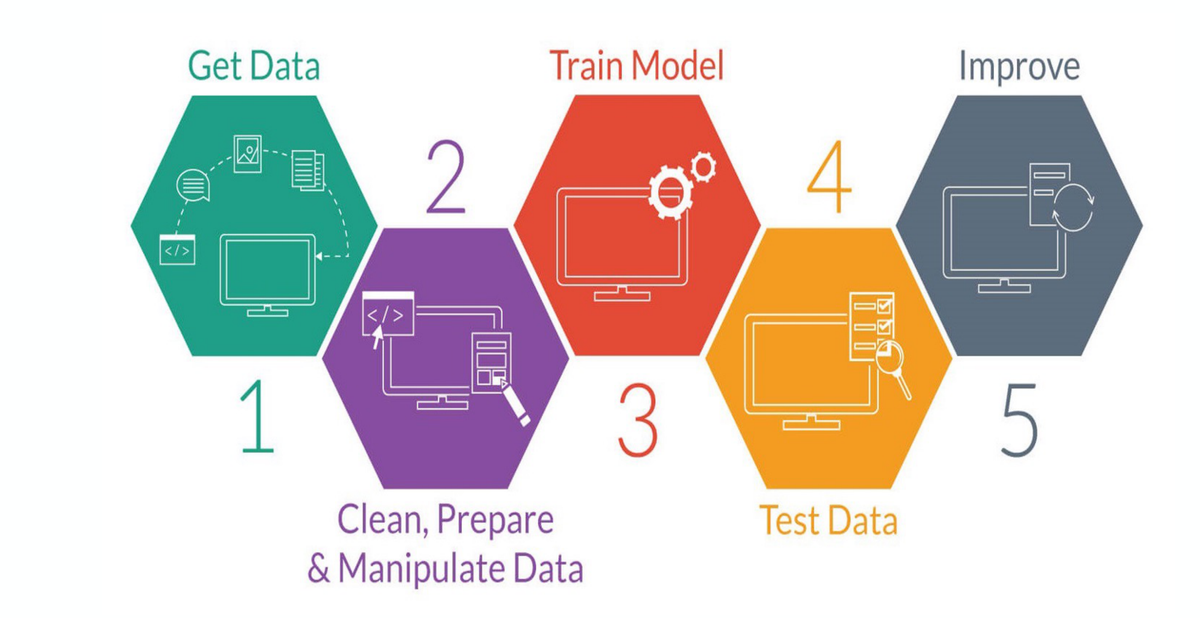
Every machine-learning project follows the same five steps. Step 2, preparing the data, usually takes most of the time.

Five steps: get data; clean, prepare and manipulate data; train model; test data; improve — The machine-learning steps: (1) get data, (2) clean, prepare and manipulate it, (3) train a model, (4) test it, (5) improve. *(From Dr. Albanna's slides.)*

Measures of data quality

Measure	Question	Example of a problem
Accuracy	Are the values correct?	Salary = −10
Completeness	Is anything missing?	Occupation left blank
Consistency	Do values agree with each other?	Age = 42 but Birthday = 03/07/2010
Believability	Can we trust the data?	Values copied from an unreliable source
Interpretability	Can we understand it?	Cryptic column codes with no documentation

2. Datasets and Data Objects

A dataset is the experience E a model learns from. The quality and diversity of the dataset decide how well the model generalizes. A dataset is made of data objects; each object is described by attributes.

Data object = an entity: a student, a customer, a patient, a transaction. Also called a sample, example, instance, data point or tuple. In a table, objects are the rows.
Attribute = a property of an object: age, name, address. Also called a feature, variable or dimension. In a table, attributes are the columns.

Types of datasets: record, graph and network, ordered, spatial and multimedia, with a document-term matrix and a transaction table — Types of datasets: **record** data (tables, document–term matrices, shopping transactions), **graphs** (the web, social networks), **ordered** data (time series, video, transaction sequences) and **spatial / multimedia** data (maps, images). *(University course slides, after J. Han, M. Kamber & J. Pei, *Data Mining: Concepts and Techniques*, 3rd ed., Morgan Kaufmann, 2012.)*

3. Attribute Types

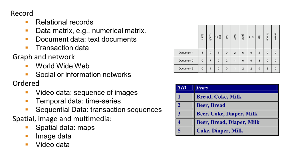
The type of an attribute decides which operations make sense on it — and which preprocessing it needs.

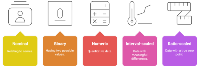
Five attribute types: nominal, binary, numeric, interval-scaled, ratio-scaled — Attribute types. *(University course slides.)*

Type	Meaning	Examples	Meaningful operations
Nominal	Names or categories, no order	Hair colour {black, blond, brown, red}; city; ID number	=, ≠ (count, mode)
Binary	Nominal with only two states, 0 and 1	Symmetric: gender (both outcomes equally important). Asymmetric: medical test (code the important outcome, “positive”, as 1)	=, ≠
Ordinal	Ordered, but the gaps between values are unknown	Size {small, medium, large}; grades; army ranks	=, ≠, <, > (median)
Interval	Numeric, equal-sized units, no true zero	Temperature in °C; calendar dates	+, − (mean)
Ratio	Numeric with a true zero	Temperature in Kelvin; length; weight; income	+, −, ×, ÷ (“twice as much”)

Why it matters

20°C is not “twice as hot” as 10°C, because 0°C is not the absence of heat (interval). 20 kg is twice 10 kg (ratio). And encoding cities as 1, 2, 3 does not make Paris “greater than” Rome — nominal attributes need one-hot encoding, not arithmetic.

4. The Major Tasks of Data Preprocessing

The four tasks as before → after. Cleaning replaces the missing age and the impossible −10 with the mean of the valid ages (25 + 35 + 30) / 3 = 30. Integration joins two sources that name the same key differently. Transformation divides by 100 so every value falls in [−1, 1]. Reduction keeps fewer rows (sampling) and fewer attributes (selection). (Adapted from Dr. Albanna's slides.)

Task	What it does
Data cleaning	Fill in missing values, smooth noisy data, identify or remove outliers, resolve inconsistencies
Data integration	Combine multiple databases, data cubes or files into one consistent store
Data transformation	Normalization (scaling to a range), aggregation, discretization, building new attributes
Data reduction	A smaller representation that gives the same or similar results: dimensionality reduction, attribute selection, sampling, compression

5. Data Cleaning and Missing Values

Data in the real world is dirty. It is incomplete (missing values), noisy (errors and outliers) and inconsistent (conflicting codes or names). Here is a dirty table with every problem labelled:

Missing value — the city is blank
Invalid value — gender “A” ∉ {M, F}
Duplicate key & format — Id 555 used twice; date not dd/mm/yyyy
Misfielded value — a country in the City column
Broken dependency — not a teacher, yet 5 students
Misspelling — “Rmoe” should be Rome

Seven kinds of dirty data in one table — each highlighted cell is a problem a model would silently learn from. (Adapted from Dr. Albanna's slides.)

Why values go missing

Equipment malfunction; a value deleted because it was inconsistent with other data; data not entered because of a misunderstanding; data not considered important at the time of entry; no record kept of changes.

How to handle missing values

Method	When to use it
Ignore the row	When the class label is missing, or only a few rows are affected. Wasteful if many rows have gaps.
Fill in manually	Tedious and usually infeasible for large data.
Global constant	Fill with “unknown”. Careful: the model may treat “unknown” as a real class.
Attribute mean (or median)	Simple and common for numeric data. Use the median if there are outliers; use the mode for categories.
Class-wise mean	Mean of the samples in the same class. Smarter, because it uses the label.
Most probable value	Predict the value with regression, a Bayesian method or a decision tree. Most accurate, most work.

Worked example — mean and class-wise mean

Ages of six customers, two missing, with a class label buys:

Customer	1	2	3	4	5	6
Age	25	?	35	40	?	30
Buys	yes	yes	no	no	no	yes

Attribute mean: (25 + 35 + 40 + 30) / 4 = 32.5 → both gaps become 32.5.

Class-wise mean: customer 2 buys = yes → mean of the “yes” ages (25 + 30) / 2 = 27.5. Customer 5 buys = no → mean of the “no” ages (35 + 40) / 2 = 37.5. Each gap now reflects its own group.

6. Noisy Data and Binning

Noise is random error in a measured variable. It comes from faulty instruments, data-entry and transmission problems, technology limits, and inconsistent naming conventions. Ways to handle it:

Binning — sort the data, split it into bins, then smooth each bin by its mean, median or boundaries.
Regression — smooth by fitting the data to a function (Module 3).
Clustering — values that fall outside every cluster are outliers (Module 10).
Computer + human inspection — the computer flags suspicious values; a person checks them.

Binning methods

Method	How bins are made	Note
Equal-width (distance)	`N` intervals of equal size: width `W = (B − A) / N`, where A and B are the lowest and highest values	Simplest, but outliers dominate and skewed data is handled badly
Equal-frequency (depth)	`N` intervals, each with about the same number of samples	Good data scaling; handles skewed data
Quantile	Bin edges at the quantiles of the data	The formal version of equal-frequency
Custom	Edges chosen from domain knowledge	Ages → child, teenager, adult, senior

The 12 price values split into equal-width bins (3, 4, 5 values) and equal-frequency bins (4, 4, 4 values) — The same 12 prices binned two ways. Equal-width bins have equal ranges but unequal counts (3, 4, 5); equal-frequency bins have equal counts (4, 4, 4) but unequal ranges.

Worked example 1 — equal-width bins, smoothing by means

Data: {1, 3, 5, 7, 9, 11, 13, 15, 17, 19}, 3 bins. Width = (19 − 1) / 3 = 6, so the bins are [1, 7], (7, 13], (13, 19].

Bin 1 = {1, 3, 5, 7}: mean 16 / 4 = 4. Bin 2 = {9, 11, 13}: mean 33 / 3 = 11. Bin 3 = {15, 17, 19}: mean 51 / 3 = 17.

Smoothed data: {4, 4, 4, 4, 11, 11, 11, 17, 17, 17}.

Worked example 2 — equal-frequency bins, means and boundaries

Example from Han, Kamber & Pei, Data Mining: Concepts and Techniques.

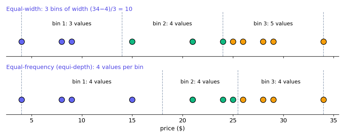
Sorted prices ($): 4, 8, 9, 15, 21, 21, 24, 25, 26, 28, 29, 34. Three bins of 4 values each:

Bin	Values	Smoothing by bin means	Smoothing by bin boundaries
1	4, 8, 9, 15	36 / 4 = 9 → 9, 9, 9, 9	4, 4, 4, 15
2	21, 21, 24, 25	91 / 4 = 22.75 ≈ 23 → 23, 23, 23, 23	21, 21, 25, 25
3	26, 28, 29, 34	117 / 4 = 29.25 ≈ 29 → 29, 29, 29, 29	26, 26, 26, 34

Smoothing by boundaries: the bin's minimum and maximum are its boundaries, and every other value moves to the closest boundary. In bin 1, 8 is 4 away from 4 and 7 away from 15, so it becomes 4; 9 is 5 away from 4 and 6 away from 15, so it also becomes 4. In bin 3, 29 is 3 away from 26 and 5 away from 34, so it becomes 26.

7. Data Transformation and Normalization

Data transformation maps the values of an attribute to a new set of values. Methods include smoothing (removing noise), attribute construction (building new attributes from old ones), aggregation (summarizing, e.g. daily → monthly sales), normalization and discretization.

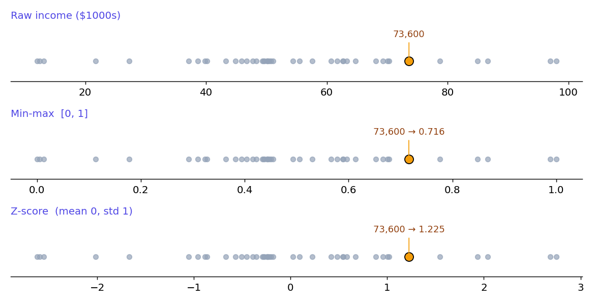
Why normalize? Attributes measured on different scales distort any method that uses distances or gradients. An income of 73,600 would swamp an age of 35 in a distance calculation. Normalization puts every attribute on a comparable scale.

Min-max normalization

Map the range [min_A, max_A] of attribute A linearly onto a new range, usually [0, 1]:

\[ v' = \frac{v - \min_A}{\max_A - \min_A}\,(\mathrm{new\_max}_A - \mathrm{new\_min}_A) + \mathrm{new\_min}_A \]

Z-score normalization (standardization)

Subtract the mean μ_A and divide by the standard deviation σ_A. The result has mean 0 and standard deviation 1, and it is not bounded, so it copes better with outliers than min-max:

\[ v' = \frac{v - \mu_A}{\sigma_A} \]

Worked example

Example from Han, Kamber & Pei, Data Mining: Concepts and Techniques.

Income ranges from $12,000 to $98,000, with mean μ = 54,000 and standard deviation σ = 16,000. Normalize v = $73,600.

Min-max to [0, 1]: (73,600 − 12,000) / (98,000 − 12,000) = 61,600 / 86,000 = 0.716.

Z-score: (73,600 − 54,000) / 16,000 = 19,600 / 16,000 = 1.225 — this income is 1.225 standard deviations above the mean.

The same incomes on the raw scale, min-max scale and z-score scale, with 73,600 highlighted — Normalization changes the scale, not the shape: the points keep their order and relative spacing. $73,600 becomes 0.716 under min-max and 1.225 under z-score.

Discretization

Discretization divides the range of a continuous attribute into intervals and replaces the values with interval labels (e.g. age → young / middle-aged / senior). It reduces the data and is required by algorithms that need categories, such as ID3 (Module 6). Methods: binning and histogram analysis (top-down, unsupervised), clustering, decision-tree splits (supervised), and correlation analysis (bottom-up merging).

8. Data Reduction

The curse of dimensionality

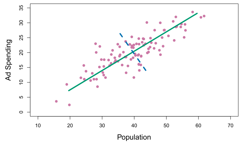
As the number of attributes grows, the data becomes increasingly sparse: distances between points become less meaningful, which hurts clustering and outlier detection, and the number of possible combinations explodes. Dimensionality reduction avoids this curse, removes irrelevant features and noise, and cuts the time and space needed for learning.

Principal Component Analysis (PCA)

PCA finds new axes — principal components — along which the data varies most. Keeping only the first few components keeps most of the information with far fewer dimensions.

Population vs ad spending for 100 cities with the first principal component as a green line and the second as a blue dashed line — Population and ad spending for 100 cities. The first principal component (green) captures most of the variation; the second (blue dashed) captures what is left. Projecting onto the green line turns two attributes into one. *(Textbook T1: James, Witten, Hastie & Tibshirani, An Introduction to Statistical Learning with Applications in Python, Springer 2023, Figure 6.14.)*

Attribute subset selection

Drop attributes that add nothing:

Redundant attributes duplicate the information in others — the purchase price of a product and the sales tax paid on it.
Irrelevant attributes carry no useful information for the task — a student's ID number when predicting GPA.

Sampling

Use a small sample s to represent the whole dataset of size N, so learning runs much faster.

Method	How it works
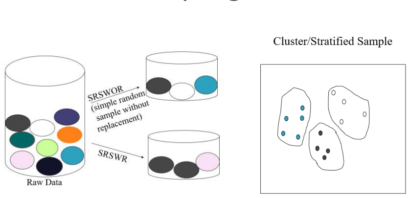
Simple random sampling	Every item has the same probability of being chosen
Without replacement (SRSWOR)	Once chosen, an object is removed — it cannot be picked again
With replacement (SRSWR)	A chosen object stays in the population and can be picked again (used by bagging, Module 11)
Stratified sampling	Split the data into groups (strata) and sample each in proportion, so every group keeps the same percentage as in the full data

Raw data sampled with and without replacement, and a cluster/stratified sample — Sampling without replacement (SRSWOR) and with replacement (SRSWR), and a cluster/stratified sample. *(University course slides; figure from Han, Kamber & Pei, *Data Mining: Concepts and Techniques*.)*

9. Imbalanced Data

A dataset is imbalanced when some classes are badly under-represented. In fraud detection, 99.9% of transactions may be legitimate and only 0.1% fraudulent.

The accuracy trap

A model that always says “legitimate” scores 99.9% accuracy — and catches no fraud at all. On imbalanced data, accuracy says nothing about the minority class; use precision, recall and F1 instead (Module 5).

Undersampling — remove samples from the majority class.
Oversampling — duplicate (or synthesize, e.g. SMOTE) samples of the minority class.
Stratified splits — keep the class ratio the same in the training and test sets.
Class weights — make mistakes on the minority class cost more during training.

10. Splitting the Data: Holdout and Cross-Validation

The last preprocessing step is to split the data so the model is tested on data it never saw (Module 1, Section 11).

Holdout — randomly split into two independent sets, e.g. 2/3 for training and 1/3 for testing. Repeating the holdout with different random splits gives random subsampling.
k-fold cross-validation (k = 10 is the most popular) — split into k mutually exclusive folds of about equal size; in round i, fold i is the test set and the others train.
Leave-one-out — k = number of samples; for small datasets.
Stratified cross-validation — each fold keeps about the same class distribution as the full data. Essential for imbalanced data.

Avoid data leakage

Compute the mean for imputation, the min/max for scaling, and so on, from the training set only, then apply the same numbers to the test set. Using the test set to fit the preprocessing leaks information about it into the model and makes the test score look better than it really is.

Python Lab: Preprocessing with pandas and scikit-learn

Run this in Google Colab. It repeats every worked example on this page: fixing inconsistent names, imputing missing values, min-max and z-score scaling, both binning methods, and a stratified split.

import numpy as np, pandas as pd
from sklearn.impute import SimpleImputer
from sklearn.preprocessing import MinMaxScaler, StandardScaler, KBinsDiscretizer
from sklearn.model_selection import train_test_split

# A small dirty table: missing values and an inconsistent city name
df = pd.DataFrame({
    "age":    [25, np.nan, 35, 40, np.nan, 30],
    "income": [12000, 98000, 73600, 54000, np.nan, 40000],
    "city":   ["Rome", "rome", "Paris", None, "Paris", "Rome"],
})
print(df.isna().sum())                                   # age 2, income 1, city 1

# 1. Cleaning: fix the naming inconsistency, then fill the gaps
df["city"] = df["city"].str.title()                        # "rome" -> "Rome"
df["city"] = df["city"].fillna(df["city"].mode()[0])        # most frequent city
df[["age", "income"]] = SimpleImputer(strategy="mean").fit_transform(df[["age", "income"]])

# 2. Normalization: 73,600 -> 0.716 with min-max (min 12,000, max 98,000)
df["income_minmax"] = MinMaxScaler().fit_transform(df[["income"]])
df["income_z"]      = StandardScaler().fit_transform(df[["income"]])
print(df.round(3))

# 3. Binning the 12 prices: equal-width ("uniform") vs equal-frequency ("quantile")
price = np.array([4, 8, 9, 15, 21, 21, 24, 25, 26, 28, 29, 34]).reshape(-1, 1)
for strategy in ["uniform", "quantile"]:
    kb = KBinsDiscretizer(n_bins=3, encode="ordinal", strategy=strategy)
    bins = kb.fit_transform(price).ravel().astype(int)
    print(strategy, bins, kb.bin_edges_[0].round(2))
# uniform  edges 4, 14, 24, 34  (scikit-learn puts a value equal to an edge, like 24, in the upper bin)
# quantile edges 4, 19, 25.33, 34 -> bins {4,8,9,15} {21,21,24,25} {26,28,29,34}

# 4. Imbalanced data: a stratified split keeps the 5% fraud rate in both sets
X = np.arange(100).reshape(-1, 1)
y = np.array([0] * 95 + [1] * 5)
X_tr, X_te, y_tr, y_te = train_test_split(X, y, test_size=0.2, stratify=y, random_state=0)
print("fraud rate train/test:", y_tr.mean(), y_te.mean())         # 0.05 0.05

Try it

Remove stratify=y and run the split with a few different random_state values. How often does the test set end up with no fraud cases at all?

Textbook Reading

From the course syllabus

T1 James et al. — ISLP, §6.3 Dimension Reduction Methods (principal components) and §12.2 Principal Components Analysis.
T2 Murphy — Probabilistic Machine Learning, §1.5 Data (§1.5.3 preprocessing discrete input data, §1.5.5 handling missing data) and §10.2.8 Standardization.

Both books are free to read online from their authors: statlearning.com (T1) and probml.github.io (T2).

Exercises

1

Name the attribute type

Classify each attribute as nominal, binary (symmetric or asymmetric), ordinal, interval or ratio: (a) blood type; (b) COVID test result; (c) customer satisfaction (1 = poor … 5 = excellent); (d) year of birth; (e) monthly salary; (f) smoker yes/no in a survey where both answers are equally important.

(a) Nominal. (b) Asymmetric binary (code “positive” as 1). (c) Ordinal — ordered, but the gap between 1 and 2 need not equal the gap between 4 and 5. (d) Interval — year 0 is not “no time”. (e) Ratio — $0 is a true zero, and $4,000 is twice $2,000. (f) Symmetric binary.

2

Fill the gaps

Exam scores: 70, ?, 85, 90, ?, 60, 75. Passed: yes, no, yes, yes, yes, no, yes. Fill the missing scores (a) with the attribute mean, (b) with the class-wise mean.

(a) Mean of the 5 known scores = (70 + 85 + 90 + 60 + 75) / 5 = 380 / 5 = 76; both gaps become 76. (b) Student 2 failed: the known “no” score is 60, so the gap becomes 60. Student 5 passed: the known “yes” scores are 70, 85, 90, 75 with mean 320 / 4 = 80, so the gap becomes 80.

3

Equal-width binning

Data: 5, 10, 11, 13, 15, 35, 50, 55, 72, 92. Make 3 equal-width bins, then smooth by bin means.

Width = (92 − 5) / 3 = 29, so the bins are [5, 34], (34, 63], (63, 92]. Bin 1 = {5, 10, 11, 13, 15}, mean 54 / 5 = 10.8. Bin 2 = {35, 50, 55}, mean 140 / 3 ≈ 46.67. Bin 3 = {72, 92}, mean 164 / 2 = 82. Smoothed: 10.8, 10.8, 10.8, 10.8, 10.8, 46.67, 46.67, 46.67, 82, 82. Note how unequal the bin counts are (5, 3, 2) — the price of equal-width bins on skewed data.

4

Equal-frequency binning and boundaries

Same data as Exercise 3. Make 2 equal-frequency bins and smooth by bin boundaries.

Bin 1 = {5, 10, 11, 13, 15}, boundaries 5 and 15: 10 is 5 from 5 and 5 from 15 (a tie — take the lower boundary by convention), 11 → 15 (4 vs 6), 13 → 15. Result: 5, 5, 15, 15, 15. Bin 2 = {35, 50, 55, 72, 92}, boundaries 35 and 92: 50 → 35 (15 vs 42), 55 → 35 (20 vs 37), 72 → 92 (37 vs 20). Result: 35, 35, 35, 92, 92.

5

Normalize a value

A house-size attribute ranges from 50 m² to 450 m², with mean 200 and standard deviation 80. Normalize 250 m² (a) by min-max to [0, 1], (b) by min-max to [−1, 1], (c) by z-score.

(a) (250 − 50) / (450 − 50) = 200 / 400 = 0.5. (b) 0.5 × (1 − (−1)) + (−1) = 0.5 × 2 − 1 = 0. (c) (250 − 200) / 80 = 0.625.

6

Spot the problem

A dataset has 10,000 patients, of whom 100 have a rare disease. A model reaches 99% accuracy. (a) Why is this not impressive? (b) How should the data be split? (c) Name two ways to rebalance the training data.

(a) Predicting “healthy” for everyone already gives 9,900 / 10,000 = 99% accuracy while missing every sick patient; check recall on the disease class. (b) With a stratified split, so the training and test sets both keep 1% positives. (c) Undersample the healthy class, or oversample (duplicate or synthesize, e.g. SMOTE) the disease class — or use class weights.

Recap & Where Next

You now know

Data quality has five measures: accuracy, completeness, consistency, believability and interpretability.
Attributes are nominal, binary, ordinal, interval or ratio, and the type decides the valid operations.
The four tasks: cleaning, integration, transformation, reduction.
Missing values are dropped, filled with a constant, a mean (overall or per class), or a predicted value; noise is smoothed by binning, regression or clustering.
Min-max maps to a fixed range; z-score gives mean 0 and standard deviation 1.
Reduce data with PCA, attribute selection and sampling; handle imbalance with resampling and stratified splits — and fit preprocessing on the training set only.

With clean data in hand we can fit our first real model. Module 3 starts supervised learning with linear regression.