Naive Bayes - Machine Learning

What You'll Learn

The probability basics: prior, conditional and joint probability, and independence
Bayes' theorem: prior, likelihood, evidence and posterior — and why a positive medical test can still mean a low chance of disease
The MAP rule and the naïve (class-conditional independence) assumption
The learning and test phases of Naïve Bayes, worked by hand on PlayTennis
The zero-frequency problem and Laplace smoothing
The three types: Gaussian, Multinomial and Bernoulli Naïve Bayes

Prerequisites: Module 6 (we reuse the PlayTennis data) and basic probability.

1. Probability Basics

Probabilistic classifiers pick the most likely class for an observation by modelling how the features are distributed in each class. They combine prior knowledge with observed data.

Concept	Notation	Meaning
Prior probability	`P(A)`	Probability of A before seeing any evidence
Conditional probability	`P(A \| B)`	Probability of A given that B has happened
Joint probability	`P(A, B)`	Probability that A and B both happen
Product (chain) rule	`P(A, B) = P(A \| B) P(B) = P(B \| A) P(A)`	Links joint and conditional probability
Independence	`P(A, B) = P(A) P(B)`	Knowing B tells us nothing about A: `P(A \| B) = P(A)`

From the PlayTennis data

Of the 14 days, 9 are “Yes” and 5 are Sunny; 2 days are both Sunny and Yes. Prior P(Yes) = 9/14 = 0.64. Joint P(Sunny, Yes) = 2/14. Conditional P(Sunny | Yes) = 2/9 = 0.22 — and indeed P(Sunny | Yes) P(Yes) = (2/9)(9/14) = 2/14.

2. Bayes' Theorem

Writing the product rule both ways and dividing gives Bayes' theorem, which turns P(data | hypothesis) — easy to estimate — into P(hypothesis | data) — what we actually want:

\[ P(h \mid D) = \frac{P(D \mid h)\,P(h)}{P(D)} \qquad\qquad \text{posterior} = \frac{\text{likelihood} \times \text{prior}}{\text{evidence}} \]

Term	Name	Meaning
`P(h)`	Prior	How probable hypothesis h is before seeing the data
`P(D \| h)`	Likelihood	How probable the data is if h is true
`P(D)`	Evidence	How probable the data is overall: `Σ_h P(D \| h) P(h)`
`P(h \| D)`	Posterior	How probable h is after seeing the data

The posterior grows with the likelihood and with the prior, and shrinks when the evidence is common anyway.

Example 1 — fire and smoke

Example from Math is Fun, “Bayes' Theorem”.

Dangerous fires are rare (1%), smoke is fairly common (10%, thanks to barbecues), and 90% of dangerous fires make smoke. If you see smoke, what is the chance of a dangerous fire?

P(Fire | Smoke) = P(Smoke | Fire) P(Fire) / P(Smoke) = (0.90 × 0.01) / 0.10 = 0.09 — 9%. Low, but still worth checking.

3. A Medical Test: Why the Prior Matters

A population may or may not have cancer, and a screening test (such as a mammogram) returns positive or negative. If a randomly chosen patient tests positive, what is the probability that they have cancer?

	Has cancer (1%)	No cancer (99%)
Test positive	80% — true positive	9.6% — false positive
Test negative	20% — false negative	90.4% — true negative

Worked example

Example from K. Azad, “An Intuitive (and Short) Explanation of Bayes' Theorem”, BetterExplained.

P(c) = 0.01, P(¬c) = 0.99, P(+ | c) = 0.80, P(+ | ¬c) = 0.096.

True positives: P(+ | c) P(c) = 0.80 × 0.01 = 0.008. False positives: P(+ | ¬c) P(¬c) = 0.096 × 0.99 = 0.09504. Evidence: P(+) = 0.008 + 0.09504 = 0.10304.

Posterior: P(c | +) = 0.008 / 0.10304 = 0.0776, and P(¬c | +) = 0.9224.

A positive mammogram means only a 7.8% chance of cancer, not 80% (the test's sensitivity). Because the disease is rare and the false-positive rate (9.6%) is high, most positive results come from healthy people.

The same calculation with counts instead of probabilities. Out of 10,000 people, the 1% with cancer produce 80 true positives; the 99% without cancer produce about 950 false positives. A positive result is far more likely to be a false alarm.

4. Bayes' Theorem for Classification: The MAP Rule

For classification, the hypothesis is the class y and the data is the feature vector X = (x₁, …, x_n):

\[ P(y \mid x_1, \dots, x_n) = \frac{P(x_1, \dots, x_n \mid y)\,P(y)}{P(x_1, \dots, x_n)} \]

We choose the class with the largest posterior — the maximum a posteriori (MAP) class. The denominator P(X) is the same for every class, so it can be ignored when comparing:

\[ y_{MAP} = \arg\max_{y}\; P(x_1, \dots, x_n \mid y)\,P(y) \]

The problem

Estimating the full joint likelihood P(x₁, …, x_n | y) needs a probability for every combination of feature values. With just 4 PlayTennis attributes there are 3 × 3 × 2 × 2 = 36 combinations per class, and only 14 days of data. With 30 binary features there are over a billion. We cannot count them all.

5. The Naïve Bayes Classifier

Naïve Bayes makes one simplifying — “naïve” — assumption: the features are independent of one another given the class (class-conditional independence). The joint likelihood then factors into one small term per feature:

\[ P(x_1, \dots, x_n \mid y) = \prod_{i=1}^{n} P(x_i \mid y) \qquad\Longrightarrow\qquad y_{NB} = \arg\max_{y}\; P(y) \prod_{i=1}^{n} P(x_i \mid y) \]

The naïve Bayes model. The class generates each feature on its own; once the class is known, the features are assumed not to influence one another. That is what lets the joint likelihood factor into one small table per feature.

Two phases

Learning phase: from the training set, estimate every prior P(y) and every conditional P(x_i = v | y) by counting. The output is one conditional probability table per attribute.
Test phase: for a new instance X', look up its values in the tables, multiply, and assign the class with the largest score (the MAP rule).

The assumption is rarely exactly true (humidity and outlook are related), yet Naïve Bayes is competitive with far more complex classifiers even when the assumption is violated: it only needs the ranking of the classes to be right, not the exact probabilities.

6. Worked Example: PlayTennis

The same 14 days as Module 6 (9 Yes, 5 No), from T. M. Mitchell, Machine Learning, 1997.

1

Learning phase: priors and conditional probability tables

P(Yes) = 9/14, P(No) = 5/14. Each table entry counts how often a value occurs within a class:

Outlook	Yes	No
Sunny	2/9	3/5
Overcast	4/9	0/5
Rain	3/9	2/5

Temp.	Yes	No
Hot	2/9	2/5
Mild	4/9	2/5
Cool	3/9	1/5

Humidity	Yes	No
High	3/9	4/5
Normal	6/9	1/5

Wind	Yes	No
Strong	3/9	3/5
Weak	6/9	2/5

2

Test phase: classify a new day

X' = (Outlook = Sunny, Temperature = Cool, Humidity = High, Wind = Strong).

\[ \begin{aligned} \text{Yes:}&\quad P(\text{Sunny}|\text{Yes})\,P(\text{Cool}|\text{Yes})\,P(\text{High}|\text{Yes})\,P(\text{Strong}|\text{Yes})\,P(\text{Yes}) = \tfrac{2}{9}\cdot\tfrac{3}{9}\cdot\tfrac{3}{9}\cdot\tfrac{3}{9}\cdot\tfrac{9}{14} = 0.0053 \\[6pt] \text{No:}&\quad P(\text{Sunny}|\text{No})\,P(\text{Cool}|\text{No})\,P(\text{High}|\text{No})\,P(\text{Strong}|\text{No})\,P(\text{No}) = \tfrac{3}{5}\cdot\tfrac{1}{5}\cdot\tfrac{4}{5}\cdot\tfrac{3}{5}\cdot\tfrac{5}{14} = 0.0206 \end{aligned} \]

Since 0.0206 > 0.0053, label X' as No. These scores are not yet probabilities; normalizing gives P(No | X') = 0.0206 / (0.0206 + 0.0053) = 0.795.

One attribute at a time

With Outlook alone: P(Yes | Sunny) = P(Sunny | Yes) P(Yes) / P(Sunny) = (2/9)(9/14) / (5/14) = 2/5 = 0.4 and P(No | Sunny) = (3/5)(5/14) / (5/14) = 3/5 = 0.6. Together they sum to 1, as posteriors must.

7. The Zero-Frequency Problem and Laplace Smoothing

In the PlayTennis tables, P(Overcast | No) = 0/5 = 0: no “No” day in the training data was overcast. Because Naïve Bayes multiplies, a single zero wipes out the whole score — whatever the other features say, any overcast day gets P(No | X) = 0. A value never seen with a class in a small sample is not impossible; we just have not seen it yet.

Laplace (add-one) smoothing adds a small count α (usually 1) to every value of every attribute:

\[ P(x_i = v \mid y) = \frac{\text{count}(x_i = v,\, y) + \alpha}{\text{count}(y) + \alpha\,k} \]

k is the number of distinct values of the attribute (Outlook: k = 3; Wind: k = 2). Adding αk to the denominator keeps each table summing to 1. With a large training set the extra counts make a negligible difference; with a small one they prevent zeros.

Worked example — PlayTennis with α = 1

Outlook (k = 3): P(Overcast | No) = (0 + 1) / (5 + 3) = 1/8 instead of 0; P(Sunny | No) = (3 + 1)/8 = 4/8; P(Sunny | Yes) = (2 + 1)/(9 + 3) = 3/12.

Re-scoring X' = (Sunny, Cool, High, Strong): Yes = (3/12)(4/12)(4/11)(4/11)(9/14) = 0.0071; No = (4/8)(2/8)(5/7)(4/7)(5/14) = 0.0182. Still No, now with P(No | X') = 0.72 — smoothing pulls extreme probabilities toward the middle.

Worked example — will you like a movie?

Eight movies: 5 liked, 3 not. Among liked: Comedy 2, Drama 3; Short 2, Medium 3, Long 0. Among not liked: Comedy 1, Drama 2; Short 1, Medium 1, Long 1.

(Comedy, Medium): liked = 0.4 × 0.6 × 5/8 = 0.150; not liked = (1/3)(1/3)(3/8) = 0.042 → liked.

(Comedy, Long), no smoothing: liked = 0.4 × 0 × 5/8 = 0 — the zero decides by itself. With α = 1: P(Comedy | liked) = 3/7 (k = 2), P(Long | liked) = 1/8 (k = 3) → liked = (3/7)(1/8)(5/8) = 0.033; not liked = (2/5)(2/6)(3/8) = 0.050 → not liked, now decided by all the evidence rather than one empty cell.

8. Types of Naïve Bayes

The only modelling choice is how to compute P(x_i | y). That choice gives three main variants:

Type	Features	P(x_i \| y)	Typical use
Categorical (the version above)	Discrete values	Counted from tables (+ Laplace)	PlayTennis, survey answers
Gaussian	Continuous	A normal curve per class, with that class's mean μ and standard deviation σ	Measurements: iris flowers, sensor data
Multinomial	Counts	How often each value (word) occurs in the class, smoothed	Text classification, spam filtering
Bernoulli	Binary (present / absent)	Probability that the feature is present in the class	Short texts, “does the e-mail contain this word?”

Gaussian Naïve Bayes

For a continuous attribute, split the training data by class, compute the mean μ_y and standard deviation σ_y in each class, and use the normal density as the likelihood:

\[ P(x \mid y) = \frac{1}{\sqrt{2\pi}\,\sigma_y}\, \exp\!\left(-\frac{(x - \mu_y)^2}{2\sigma_y^2}\right) \]

Two normal curves for temperature, one for Play = yes (mean 73, sd 6.2) and one for Play = no (mean 74.6, sd 7.9), with the densities at 66 marked — Numeric PlayTennis temperatures: one normal curve per class. A day at 66°F has density 0.0340 under “yes” and 0.0279 under “no”.

Worked example

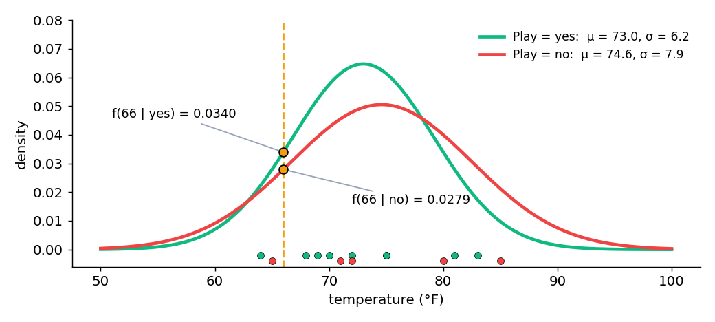
Numeric weather data from I. H. Witten, E. Frank & M. A. Hall, Data Mining: Practical Machine Learning Tools and Techniques.

Temperatures on “yes” days: 83, 70, 68, 64, 69, 75, 75, 72, 81 → μ = 73.0, σ = 6.2. On “no” days: 85, 80, 65, 72, 71 → μ = 74.6, σ = 7.9. For 66°F: f(66 | yes) = 0.0340, f(66 | no) = 0.0279. With the priors: yes 0.0340 × 9/14 = 0.0218, no 0.0279 × 5/14 = 0.0100 → yes.

9. Bayesian Learning: Updating Beliefs

Bayes' theorem is not only a classifier — it is a way to learn: start with a prior over hypotheses and update it after every observation. No hypothesis is thrown away; each just becomes more or less probable.

Worked example — bags of candy

Example from S. Russell & P. Norvig, Artificial Intelligence: A Modern Approach, Ch. 20 (Learning Probabilistic Models).

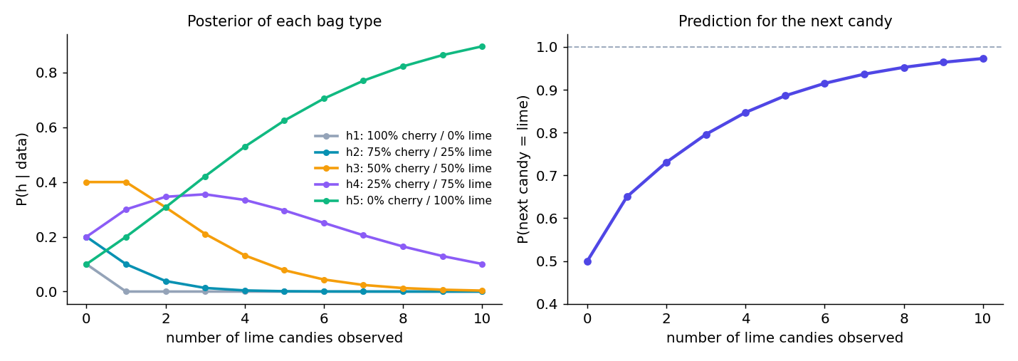
There are five kinds of candy bag: h₁ (10% of bags): 100% cherry; h₂ (20%): 75% cherry, 25% lime; h₃ (40%): 50/50; h₄ (20%): 25% cherry, 75% lime; h₅ (10%): 100% lime. We draw candies from one bag and they are all lime. What kind of bag is it, and what flavour will the next candy be?

After one lime: multiply each prior by P(lime | h) = 0, 0.25, 0.5, 0.75, 1: 0, 0.05, 0.20, 0.15, 0.10; divide by their sum 0.5 → posteriors 0, 0.10, 0.40, 0.30, 0.20.

After two limes: 0, 0.038, 0.308, 0.346, 0.308. After three: 0, 0.013, 0.211, 0.355, 0.421 — now h₅ is the most probable (MAP) bag.

Prediction: P(next = lime) = Σ P(lime | h) P(h | data): 0.50 before any candy, 0.65 after one lime, 0.73 after two, 0.80 after three, approaching 1.

Left: posterior probability of each bag type as more limes are observed; h5 rises toward 1. Right: probability that the next candy is lime rises from 0.5 toward 1. — As limes keep coming, belief shifts toward the all-lime bag h₅ (left) and the prediction for the next candy approaches certainty (right).

Bayesian learning: advantages	Drawbacks
No hypothesis is eliminated, even if it is inconsistent with some data	Prior probabilities are not always easy to estimate
Each hypothesis keeps a probability that is updated incrementally with every example	Huge computational cost in the general case (many hypotheses)
Hypotheses can make probabilistic predictions (useful for medical diagnosis)

10. Strengths and Weaknesses

Strengths	Weaknesses
Training is very fast: one pass to count each attribute in each class	The independence assumption is strong and often unrealistic
Prediction is fast: look up tables or evaluate normal curves	The probabilities it outputs are often too extreme (poorly calibrated), even when the ranking is right
Works well with small datasets and many features (text)	Zero counts need smoothing
Little memory: just the counts or means and variances	Correlated, redundant features are counted twice
Competitive accuracy; many applications (spam filtering); a good base learner for ensembles

Naïve Bayes is a generative classifier: it models how each class generates the features, P(X | y), then uses Bayes' theorem. Logistic regression (Module 4) is discriminative: it models P(y | X) directly.

Python Lab

Run this in Google Colab. Part 1 reproduces the PlayTennis calculation by counting; Part 2 repeats it with Laplace smoothing in scikit-learn; Parts 3 and 4 try Gaussian NB on measurements and Multinomial NB on text.

import numpy as np, pandas as pd
from sklearn.naive_bayes import CategoricalNB, GaussianNB, MultinomialNB
from sklearn.preprocessing import OrdinalEncoder
from sklearn.feature_extraction.text import CountVectorizer
from sklearn.datasets import load_iris
from sklearn.model_selection import cross_val_score

data = pd.DataFrame([
    ["Sunny", "Hot", "High", "Weak", "No"],      ["Sunny", "Hot", "High", "Strong", "No"],
    ["Overcast", "Hot", "High", "Weak", "Yes"],  ["Rain", "Mild", "High", "Weak", "Yes"],
    ["Rain", "Cool", "Normal", "Weak", "Yes"],   ["Rain", "Cool", "Normal", "Strong", "No"],
    ["Overcast", "Cool", "Normal", "Strong", "Yes"], ["Sunny", "Mild", "High", "Weak", "No"],
    ["Sunny", "Cool", "Normal", "Weak", "Yes"],  ["Rain", "Mild", "Normal", "Weak", "Yes"],
    ["Sunny", "Mild", "Normal", "Strong", "Yes"], ["Overcast", "Mild", "High", "Strong", "Yes"],
    ["Overcast", "Hot", "Normal", "Weak", "Yes"], ["Rain", "Mild", "High", "Strong", "No"]],
    columns=["Outlook", "Temp", "Humidity", "Wind", "Play"])
X_cols = ["Outlook", "Temp", "Humidity", "Wind"]

# ---- Part 1: Naive Bayes by counting (no smoothing) ----
def score(df, x, label):
    sub = df[df.Play == label]
    s = len(sub) / len(df)                                  # prior P(y)
    for col, val in zip(X_cols, x):
        s *= (sub[col] == val).mean()                      # times P(x_i | y)
    return s

x_new = ["Sunny", "Cool", "High", "Strong"]
s_yes, s_no = score(data, x_new, "Yes"), score(data, x_new, "No")
print(f"score(Yes) = {s_yes:.4f}   score(No) = {s_no:.4f}   P(No | x) = {s_no / (s_yes + s_no):.3f}")
# score(Yes) = 0.0053   score(No) = 0.0206   P(No | x) = 0.795

# ---- Part 2: scikit-learn with Laplace smoothing (alpha = 1) ----
enc = OrdinalEncoder()
X = enc.fit_transform(data[X_cols])
nb = CategoricalNB(alpha=1.0).fit(X, data.Play)
x_enc = enc.transform(pd.DataFrame([x_new], columns=X_cols))
print("Laplace-smoothed P(No | x) =", nb.predict_proba(x_enc)[0, 0].round(3), "->", nb.predict(x_enc)[0])   # 0.72 -> No

# ---- Part 3: Gaussian NB on continuous measurements ----
Xi, yi = load_iris(return_X_y=True)
print("Gaussian NB on iris, 10-fold accuracy:", cross_val_score(GaussianNB(), Xi, yi, cv=10).mean().round(3))  # 0.953

# ---- Part 4: Multinomial NB for text (a tiny spam filter) ----
texts = ["win money now", "cheap money offer", "win a cheap prize now",
         "meeting at noon", "project meeting notes", "lunch at noon tomorrow"]
labels = ["spam", "spam", "spam", "ham", "ham", "ham"]
vec = CountVectorizer()                                     # word counts per message
mnb = MultinomialNB(alpha=1.0).fit(vec.fit_transform(texts), labels)
for t in ["cheap prize money", "notes for the meeting"]:
    print(f"{t!r:26s} -> {mnb.predict(vec.transform([t]))[0]}")   # spam, ham

Try it

In Part 1, classify ["Overcast", "Mild", "High", "Strong"]: what is score(No), and why? Then compare with Part 2's smoothed model. In Part 4, add a few messages of your own and see how the filter's decisions change.

Textbook Reading

From the course syllabus

T1 James et al. — ISLP, §4.4.4 Naive Bayes (and §4.4 on generative models for classification).
T2 Murphy — Probabilistic Machine Learning, §2.3 Bayes' rule (including the medical-testing example) and §9.3 Naive Bayes classifiers (including Bayesian/Laplace smoothing of the counts).

Both books are free to read online from their authors: statlearning.com (T1) and probml.github.io (T2).

Exercises

1

A screening test

A disease affects 2% of people. A test detects it 90% of the time and gives a false positive 5% of the time. A person tests positive. What is the probability they have the disease?

True positives = 0.90 × 0.02 = 0.018; false positives = 0.05 × 0.98 = 0.049; P(+) = 0.067. P(disease | +) = 0.018 / 0.067 = 0.269 — about 27%. In 10,000 people: 200 sick → 180 positive; 9,800 healthy → 490 positive; 180 / 670 = 27%.

2

Classify a new day

Use the PlayTennis tables (no smoothing) to classify (Rain, Hot, High, Weak), and give P(No | X).

Yes: (3/9)(2/9)(3/9)(6/9)(9/14) = 0.0106. No: (2/5)(2/5)(4/5)(2/5)(5/14) = 0.0183. Predict No; P(No | X) = 0.0183 / 0.0289 = 0.63.

3

Spot and fix the zero

Classify (Overcast, Mild, High, Strong) (a) without smoothing, (b) with Laplace smoothing α = 1. Why is (a) a problem even though the predicted class is reasonable?

(a) Yes: (4/9)(4/9)(3/9)(3/9)(9/14) = 0.0141; No: (0/5)(…) = 0 → Yes with P = 1. The problem: Humidity = High and Wind = Strong both point toward No, but the single zero for Overcast silences them and claims total certainty. (b) Yes: (5/12)(5/12)(4/11)(4/11)(9/14) = 0.0148; No: (1/8)(3/8)(5/7)(4/7)(5/14) = 0.0068 → Yes with P = 0.68 — the same class, but an honest level of confidence.

4

Which Naïve Bayes?

Choose the variant for: (a) classifying news articles from word counts; (b) predicting a flower species from petal lengths in cm; (c) filtering SMS messages from which keywords are present; (d) predicting loan approval from employment type and marital status.

(a) Multinomial. (b) Gaussian. (c) Bernoulli (presence/absence). (d) Categorical (counted tables with Laplace smoothing).

5

Gaussian likelihood

Using the temperature curves of Section 8 (yes: μ = 73, σ = 6.2; no: μ = 74.6, σ = 7.9) and the priors 9/14 and 5/14, classify a day of 85°F. (Densities: f(85 | yes) = 0.0097, f(85 | no) = 0.0212.)

Yes: 0.0097 × 9/14 = 0.0063; No: 0.0212 × 5/14 = 0.0076 → No. At 85°F the wider “no” curve has more density than the narrow “yes” curve, enough to overturn the prior.

6

Update the candy posterior

Starting from the priors (0.1, 0.2, 0.4, 0.2, 0.1), compute the posteriors of the five bags after drawing one cherry candy. Which bag can be ruled out?

P(cherry | h) = 1, 0.75, 0.5, 0.25, 0. Products: 0.10, 0.15, 0.20, 0.05, 0; sum 0.5. Posteriors: 0.20, 0.30, 0.40, 0.10, 0. The all-lime bag h₅ is ruled out (posterior 0); P(next = cherry) = 0.2(1) + 0.3(0.75) + 0.4(0.5) + 0.1(0.25) = 0.65.

Recap & Where Next

You now know

Bayes' theorem: posterior = likelihood × prior / evidence; rare events stay unlikely even after a positive test.
Naïve Bayes assumes the features are independent given the class, so P(y | X) ∝ P(y) Π P(x_i | y), and picks the MAP class.
Learning = counting (or means and variances); testing = looking up and multiplying.
A zero count wipes out the product; Laplace smoothing (count + α) / (n + αk) fixes it.
Categorical, Gaussian, Multinomial and Bernoulli NB differ only in how they model P(x_i | y).

Logistic regression, trees and Naïve Bayes each draw a boundary in their own way. Module 8 asks a geometric question: of all the lines that separate two classes, which one is best? The answer is the support vector machine.