Decision Trees (ID3) - Machine Learning

What You'll Learn

The parts of a decision tree and how to turn a tree into IF–THEN rules
Entropy as a measure of impurity, and information gain as the reduction in entropy after a split
The ID3 algorithm: top-down, greedy, one attribute at a time
Two complete worked examples by hand: PlayTennis and “Is the car fast?”
How to split on a continuous attribute with a threshold
Why trees overfit, and how pruning fixes it

Prerequisites: Modules 1, 2 (attribute types, discretization) and 5 (accuracy and cross-validation). You need logarithms in base 2: log₂(x) = ln(x) / ln(2).

1. What Is a Decision Tree?

A decision tree classifies an example by asking a series of questions about its attributes, one at a time, until it reaches an answer. It is one of the most widely used and practical methods of inductive inference — learning general rules from specific examples.

Part	Role
Root node	The first question, at the top; it holds the whole training set
Decision (internal) node	Tests one attribute
Branch	One value (or range of values) of the tested attribute
Leaf node	Assigns a class; ideally its examples are all of one class (homogeneous)

To classify a new example, start at the root, follow the branch that matches the example's value, and repeat until you reach a leaf. The tree for PlayTennis (Section 6) asks first about the outlook: overcast → play; sunny → look at the humidity; rain → look at the wind.

A tree is a set of rules

Every path from the root to a leaf is one IF–THEN rule; the tree is the OR of its paths:

R1: IF Outlook = Sunny    AND Humidity = High    THEN PlayTennis = No
R2: IF Outlook = Sunny    AND Humidity = Normal  THEN PlayTennis = Yes
R3: IF Outlook = Overcast                        THEN PlayTennis = Yes
R4: IF Outlook = Rain     AND Wind = Strong      THEN PlayTennis = No
R5: IF Outlook = Rain     AND Wind = Weak        THEN PlayTennis = Yes

When to use a decision tree

Examples are described by attribute–value pairs (categorical, or numeric with thresholds).
The target is discrete (classification) — regression trees also exist (Section 10).
The answer may need a disjunction (“this OR that”), which trees express naturally.
The training data may be noisy or have missing values.
Typical uses: medical or equipment diagnosis, credit-risk analysis, many NLP tasks — anywhere the decision must be explained.

2. Learning a Tree Top-Down

Finding the smallest tree that fits the data is NP-hard, so every practical algorithm is greedy: build the tree from the top down, choose the best attribute for the current node, split, and never go back. Algorithms include Hunt's algorithm (one of the earliest), CART, ID3, C4.5, SLIQ and SPRINT.

ID3 — Iterative Dichotomiser 3

Invented by J. Ross Quinlan in 1979. It uses Shannon's information theory (1948) to choose, at each node, the attribute with the highest information gain, and builds the tree top-down with no backtracking.

1

Pick the best attribute

A ← the attribute that best separates the classes at this node; make it the decision attribute.

2

Branch

Create one child for each value of A and send each training example down the branch that matches its value.

3

Stop or repeat

If all examples at a child have the same class, it becomes a leaf. Otherwise repeat steps 1–3 on that child, using only the attributes not yet used on its path.

The key decision is step 1. To make it we need a way to measure how mixed — how impure — a set of examples is.

3. Impurity and Entropy

A group where every example has the same class is pure: there is nothing left to learn. A 50/50 group is as impure as it can be. The standard measure is entropy, from information theory:

\[ \begin{aligned} \text{Entropy}(S) &= -\sum_{i=1}^{c} p_i \log_2 p_i \\[6pt] \text{two classes:}\quad \text{Entropy}(S) &= -p_+\log_2 p_+ - p_-\log_2 p_- \end{aligned} \]

p_i is the proportion of examples of class i in S (by convention 0 · log 0 = 0). Entropy is the expected number of bits needed to encode the class of a randomly drawn member of S: a pure set needs 0 bits, a 50/50 set needs a full bit.

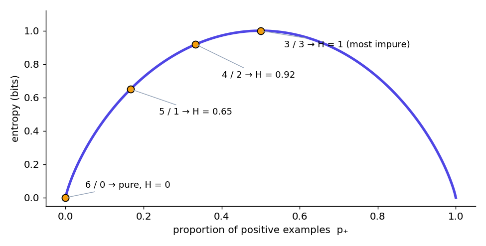
Entropy of a two-class set as a function of the proportion of positives: 0 at the ends, 1 at 0.5, with 6/0, 5/1, 4/2 and 3/3 marked — Two-class entropy is 0 for a pure set and peaks at 1 bit for a 50/50 set. The marked points are six-example groups.

Worked examples

Group of 6	p(C1)	p(C2)	Entropy
0 / 6	0	1	`−0 − 1·log₂1 = 0` (pure)
1 / 5	1/6	5/6	`−(1/6)log₂(1/6) − (5/6)log₂(5/6) = 0.65`
2 / 4	2/6	4/6	`−(2/6)log₂(2/6) − (4/6)log₂(4/6) = 0.92`
3 / 3	1/2	1/2	`−0.5·log₂0.5 − 0.5·log₂0.5 = 1` (most impure)

A larger group: 16 green circles and 14 pink crosses (30 in all): −(16/30)log₂(16/30) − (14/30)log₂(14/30) = 0.997 — almost maximally mixed.

4. Information Gain

Information gain is the drop in entropy when a set is split on an attribute A: the parent's entropy minus the weighted average entropy of the children. The attribute with the largest gain gives the most homogeneous branches and becomes the decision node.

\[ \text{Gain}(S, A) = \text{Entropy}(S) - \sum_{v \in \text{Values}(A)} \frac{|S_v|}{|S|}\,\text{Entropy}(S_v) \]

S_v is the subset of S where A has the value v. A branch with entropy 0 is a leaf; any other branch is split again, recursively, until all data is classified.

Which attribute should split the 14 days? Each child’s entropy is weighted by its share of the examples and subtracted from the parent’s 0.940. Humidity leaves purer children (gain 0.151) than Wind (0.048).

Worked example — 30 examples

Parent: 16 circles, 14 crosses → entropy 0.997. A split sends 17 examples left (13 circles, 4 crosses: entropy 0.787) and 13 right (1 circle, 12 crosses: entropy 0.391).

Weighted child entropy = (17/30)(0.787) + (13/30)(0.391) = 0.446 + 0.169 = 0.615. Gain = 0.997 − 0.615 = 0.38.

Worked example — two candidate attributes

S = [29+, 35−], entropy 0.99. Attribute A1 splits it into [21+, 5−] (entropy 0.71) and [8+, 30−] (entropy 0.74): Gain = 0.99 − (26/64)(0.71) − (38/64)(0.74) = 0.27. Attribute A2 splits it into [18+, 33−] (0.94) and [11+, 2−] (0.62): Gain = 0.99 − (51/64)(0.94) − (13/64)(0.62) = 0.12. Choose A1.

5. The ID3 Algorithm

ID3(X, T, Attrs)        # X: training examples, T: target attribute, Attrs: other attributes
    create a Root node
    if all examples in X are +:   return Root labelled +
    if all examples in X are -:   return Root labelled -
    if Attrs is empty:            return Root labelled with the most common value of T in X
    A ← the attribute in Attrs with the highest Gain(X, A)
    Root tests A
    for each value v of A:
        add a branch below Root for the test A = v
        X_v ← the examples in X with A = v
        if X_v is empty:
            add a leaf labelled with the most common value of T in X
        else:
            add the subtree ID3(X_v, T, Attrs - {A})
    return Root

Each attribute is used at most once on any path, so the recursion always ends. When the attributes run out before a node is pure, the leaf takes the majority class — you will see this in the car example.

6. Worked Example 1: PlayTennis

Fourteen days, four attributes, and whether tennis was played (9 yes, 5 no). The dataset and the ID3 walk-through are from T. M. Mitchell, Machine Learning, McGraw-Hill, 1997 (Table 3.2).

Day	Outlook	Temp.	Humidity	Wind	Play
D1	Sunny	Hot	High	Weak	No
D2	Sunny	Hot	High	Strong	No
D3	Overcast	Hot	High	Weak	Yes
D4	Rain	Mild	High	Weak	Yes
D5	Rain	Cool	Normal	Weak	Yes
D6	Rain	Cool	Normal	Strong	No
D7	Overcast	Cool	Normal	Strong	Yes
D8	Sunny	Mild	High	Weak	No
D9	Sunny	Cool	Normal	Weak	Yes
D10	Rain	Mild	Normal	Weak	Yes
D11	Sunny	Mild	Normal	Strong	Yes
D12	Overcast	Mild	High	Strong	Yes
D13	Overcast	Hot	Normal	Weak	Yes
D14	Rain	Mild	High	Strong	No

1

Entropy of the whole set

S = [9+, 5−]: Entropy(S) = −(9/14)log₂(9/14) − (5/14)log₂(5/14) = 0.940.

2

Gain of every attribute at the root

Outlook: Sunny [2+, 3−] E = 0.971; Overcast [4+, 0−] E = 0; Rain [3+, 2−] E = 0.971. Gain = 0.940 − (5/14)(0.971) − (4/14)(0) − (5/14)(0.971) = 0.247.

Attribute	Outlook	Humidity	Wind	Temperature
Gain(S, A)	0.247	0.151	0.048	0.029

Outlook wins and becomes the root. Overcast is already pure (4 yes) → leaf Yes.

3

Split the Sunny branch

S_sunny = {D1, D2, D8, D9, D11} = [2+, 3−], entropy 0.971.

Humidity: High [0+, 3−], Normal [2+, 0−] → Gain = 0.971 − (3/5)(0) − (2/5)(0) = 0.971
Temperature: Hot [0+, 2−], Mild [1+, 1−], Cool [1+, 0−] → Gain = 0.971 − (2/5)(1.0) = 0.571
Wind: Weak [1+, 2−], Strong [1+, 1−] → Gain = 0.971 − (3/5)(0.918) − (2/5)(1.0) = 0.020

Humidity separates the sunny days perfectly.

4

Split the Rain branch

S_rain = {D4, D5, D6, D10, D14} = [3+, 2−]. Wind: Weak [3+, 0−], Strong [0+, 2−] → gain 0.971, a perfect split (see Exercise 3 for the others).

The tree ID3 builds for PlayTennis. Each node shows its examples [yes+, no−] and entropy; each leaf lists the training days that reach it. Every leaf is pure, so the tree classifies all 14 days correctly.

7. Worked Example 2: Is the Car Fast?

Fifteen cars, four attributes. The Model column is dropped: it is unique for every car, so it cannot generalize.

Model	Engine	SC/Turbo	Weight	Fuel Eco	Fast
Prius	small	no	average	good	no
Civic	small	no	light	average	no
WRX STI	small	yes	average	bad	yes
M3	medium	no	heavy	bad	yes
RS4	large	no	average	bad	yes
GTI	medium	no	light	bad	no
XJR	large	yes	heavy	bad	no
S500	large	no	heavy	bad	no
911	medium	yes	light	bad	yes
Corvette	large	no	average	bad	yes
Insight	small	no	light	good	no
RSX	small	no	average	average	no
IS350	medium	no	heavy	bad	no
MR2	small	yes	average	average	no
E320	medium	no	heavy	bad	no

1

Root: entropy and gains

5 fast, 10 not: E(S) = −(5/15)log₂(5/15) − (10/15)log₂(10/15) = 0.528 + 0.390 = 0.918.

Attribute	Branches (yes / no)	Weighted entropy	Gain
Engine	small 1/5 (0.65), medium 2/3 (0.97), large 2/2 (1)	(6/15)0.65 + (5/15)0.97 + (4/15)1 = 0.85	0.068
SC/Turbo	yes 2/2 (1), no 3/8 (0.85)	(4/15)1 + (11/15)0.85 = 0.89	0.032
Weight	average 3/3 (1), light 1/3 (0.81), heavy 1/4 (0.72)	(6/15)1 + (4/15)0.81 + (5/15)0.72 = 0.86	0.061
Fuel Eco	good 0/2 (0), average 0/3 (0), bad 5/5 (1)	(10/15)1 = 0.667	0.251

Fuel Eco becomes the root. Good and average fuel economy are pure → leaves no.

2

The Bad branch (10 cars, 5 / 5, entropy 1)

Attribute	Branches (yes / no)	Gain
Engine	small 1/0 (0), medium 2/3 (0.97), large 2/2 (1)	1 − (5/10)0.97 − (4/10)1 = 0.115
SC/Turbo	yes 2/1 (0.92), no 3/4 (0.99)	1 − (3/10)0.92 − (7/10)0.99 = 0.035
Weight	average 3/0 (0), heavy 1/4 (0.72), light 1/1 (1)	1 − (5/10)0.72 − (2/10)1 = 0.439

Weight is next. Average weight is pure → leaf yes. Light (GTI, 911) splits perfectly on SC/Turbo: turbo → yes, no turbo → no.

3

The Heavy branch (5 cars, 1 / 4, entropy 0.72)

M3 (medium, no turbo, fast), XJR (large, turbo, not), S500 (large, no turbo, not), IS350 and E320 (medium, no turbo, not). Engine: large 0/2 (0), medium 1/2 (0.92) → Gain = 0.72 − (3/5)(0.92) = 0.171. SC/Turbo: yes 0/1, no 1/3 (0.81) → Gain = 0.72 − (4/5)(0.81) = 0.073. Split on Engine: large → no. The three medium cars all have no turbo, so no attribute is left to separate them → majority leaf no (the M3 is misclassified).

The finished tree for “Is the car fast?”. The Heavy branch (left as “?” in the slides) splits on Engine (gain 0.171). Large engines are all not fast; the three medium cars cannot be separated by the remaining attribute, so the leaf takes the majority class — “no” — and misclassifies the M3.

8. Continuous Attributes

ID3 needs discrete values. For a numeric attribute we create a binary test A ≤ t versus A > t and choose the best threshold t:

1

Sort

Sort the examples by the attribute's value.

2

Candidate thresholds

Take the midpoint between every pair of neighbouring values (only midpoints where the class changes can be optimal).

3

Pick the best

Compute the information gain of each candidate split and keep the largest. The numeric attribute then competes with the others like any categorical attribute.

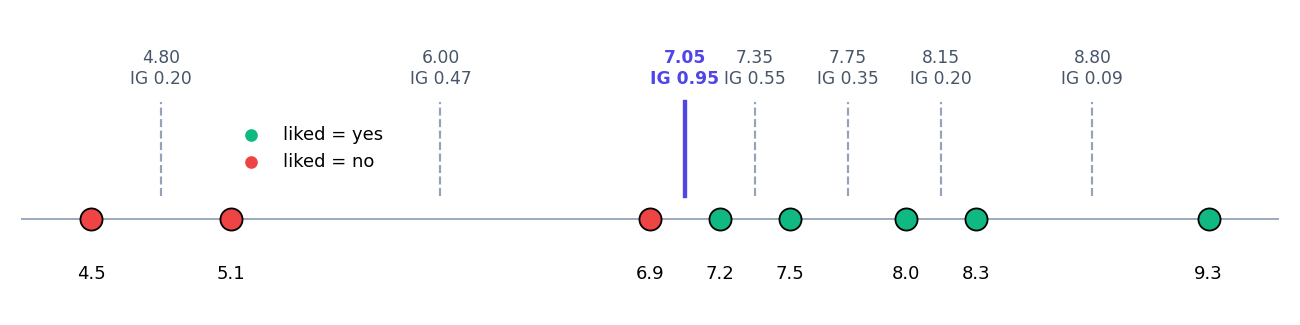
Worked example — will you like a movie?

Eight movies with their IMDb rating and whether they were liked: 7.2 yes, 9.3 yes, 5.1 no, 6.9 no, 8.3 yes, 4.5 no, 8.0 yes, 7.5 yes. Sorted: 4.5, 5.1, 6.9, 7.2, 7.5, 8.0, 8.3, 9.3. Parent entropy (5 yes, 3 no) = 0.954.

Threshold 7.05 (between 6.9 and 7.2): left = {4.5, 5.1, 6.9}, all no (entropy 0); right = {7.2, …, 9.3}, all yes (entropy 0). Gain = 0.954 − 0 = 0.954 — a perfect split. The tree is a single question: IMDb rating ≤ 7.05 → No; > 7.05 → Yes.

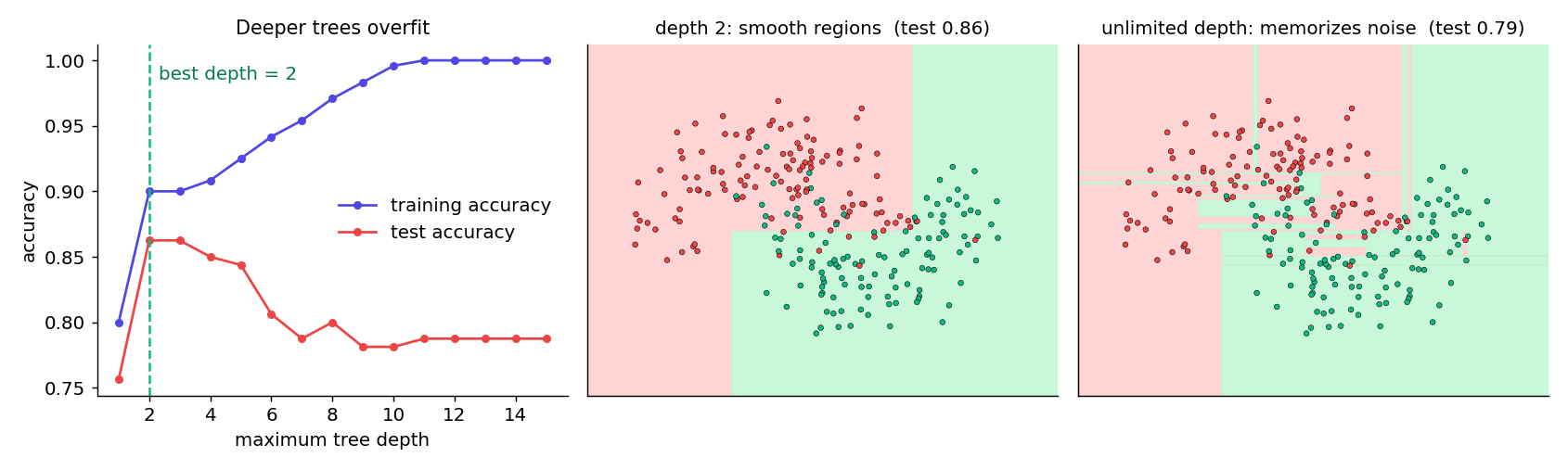
Eight movies on a rating line with seven candidate thresholds; 7.05 has the highest gain, 0.95 — Every midpoint is a candidate threshold. Only 7.05 separates the classes completely (gain 0.95); the others leave mixed groups.

9. Overfitting and Pruning

ID3 keeps splitting until every leaf is pure. On real data that means the deepest branches fit individual noisy examples — the tree memorizes the training set and generalizes badly.

Why trees overfit

Too much variance: the training data is not a representative sample, or the tree splits on features that are actually irrelevant.
Too much noise: some feature values or class labels are wrong, and the tree grows branches to fit them.
Too little data per leaf: after many splits, each leaf rests on only a handful of examples.

Left: training accuracy rises to 1 with depth while test accuracy peaks at depth 2. Middle: a depth-2 tree with simple rectangular regions. Right: an unlimited tree with many thin regions around noisy points. — **Left:** training accuracy reaches 100% as the tree deepens, but test accuracy peaks at depth 2. **Middle and right:** a tree divides the space into axis-parallel rectangles; the unlimited tree carves thin slivers around individual noisy points.

Remedy	How
Pre-pruning (stop early)	Stop growing when the depth reaches a limit, a node has too few examples, or the best gain is below a threshold.
Post-pruning (grow, then cut)	Grow the full tree, then replace subtrees by leaves when that does not hurt accuracy on a validation set (reduced-error pruning) or by trading size against error (cost-complexity pruning).
Tune on validation data	Choose the depth or pruning strength with cross-validation (Module 5), never on the training set.
Ensembles	Average many trees (random forests, boosting — Module 11).

10. Strengths, Weaknesses and Variants

Strengths	Weaknesses
Inexpensive to build, extremely fast to classify	Greedy: each split is locally best, with no global optimization
Easy to read and explain (for small trees)	Error-prone with many classes: the examples per leaf shrink quickly
Handles numeric and categorical data with little preprocessing (no scaling needed)	Expensive to train on large data: sorting and scoring every candidate split
Accuracy comparable to other methods on many simple datasets	Only axis-parallel, rectangular regions: a diagonal boundary needs a staircase of splits
Robust to noise and missing values (with care)	Unstable: a small change in the data can change the whole tree

Variants you will meet

C4.5 (Quinlan's successor to ID3) uses the gain ratio, which stops attributes with many values (like an ID number) from looking falsely good, and handles numeric attributes, missing values and pruning.
CART (used by scikit-learn) builds binary trees and usually measures impurity with the Gini index 1 − Σp_i²; it behaves very much like entropy.
Regression trees predict a number: each leaf outputs the mean target of its training examples, and splits are chosen to reduce the variance (MSE) instead of the entropy.
Practical issues: missing values (send the example down the most common branch, or down all branches with weights) and the cost of measuring an attribute (a blood test is cheap, a scan is not).

Python Lab

Run this in Google Colab. Part 1 implements entropy and information gain from scratch and reproduces the PlayTennis gains. Part 2 fits scikit-learn's tree. Part 3 chooses the depth by 10-fold cross-validation.

import numpy as np, pandas as pd
from sklearn.tree import DecisionTreeClassifier, export_text
from sklearn.datasets import load_breast_cancer
from sklearn.model_selection import cross_val_score

data = pd.DataFrame([
    ["Sunny", "Hot", "High", "Weak", "No"],      ["Sunny", "Hot", "High", "Strong", "No"],
    ["Overcast", "Hot", "High", "Weak", "Yes"],  ["Rain", "Mild", "High", "Weak", "Yes"],
    ["Rain", "Cool", "Normal", "Weak", "Yes"],   ["Rain", "Cool", "Normal", "Strong", "No"],
    ["Overcast", "Cool", "Normal", "Strong", "Yes"], ["Sunny", "Mild", "High", "Weak", "No"],
    ["Sunny", "Cool", "Normal", "Weak", "Yes"],  ["Rain", "Mild", "Normal", "Weak", "Yes"],
    ["Sunny", "Mild", "Normal", "Strong", "Yes"], ["Overcast", "Mild", "High", "Strong", "Yes"],
    ["Overcast", "Hot", "Normal", "Weak", "Yes"], ["Rain", "Mild", "High", "Strong", "No"]],
    columns=["Outlook", "Temp", "Humidity", "Wind", "Play"])

# ---- Part 1: entropy and information gain from scratch ----
def entropy(labels):
    p = labels.value_counts(normalize=True)
    return -(p * np.log2(p)).sum()

def info_gain(df, attr, target="Play"):
    weighted = sum(len(sub) / len(df) * entropy(sub[target]) for _, sub in df.groupby(attr))
    return entropy(df[target]) - weighted

print("Entropy(S) =", round(entropy(data["Play"]), 3))                      # 0.94
for a in ["Outlook", "Temp", "Humidity", "Wind"]:
    print(f"Gain(S, {a:8s}) = {info_gain(data, a):.3f}")                   # 0.247 0.029 0.152 0.048
sunny = data[data.Outlook == "Sunny"]
print({a: round(info_gain(sunny, a), 3) for a in ["Temp", "Humidity", "Wind"]})  # Humidity 0.971

# ---- Part 2: scikit-learn (CART: binary splits on one-hot columns) ----
X = pd.get_dummies(data.drop(columns="Play"))
tree = DecisionTreeClassifier(criterion="entropy", random_state=0).fit(X, data["Play"])
print(export_text(tree, feature_names=list(X.columns)))

# ---- Part 3: choose the depth by 10-fold cross-validation ----
Xb, yb = load_breast_cancer(return_X_y=True)
for depth in [1, 2, 3, 4, 6, 8, None]:
    acc = cross_val_score(DecisionTreeClassifier(max_depth=depth, random_state=0), Xb, yb, cv=10).mean()
    print(f"max_depth={str(depth):4s}  10-fold accuracy = {acc:.3f}")
# depth 2 already reaches 0.921; an unlimited tree (0.917) is no better

Try it

scikit-learn's tree in Part 2 looks different from ID3's because CART only makes binary splits (“Outlook_Overcast ≤ 0.5?”). Trace it by hand: does it make the same predictions as the ID3 tree for all 14 days? In Part 3 replace max_depth with min_samples_leaf=5 or ccp_alpha=0.01 (post-pruning).

Textbook Reading

From the course syllabus

T1 James et al. — ISLP, Ch. 8 Tree-Based Methods, §8.1 The Basics of Decision Trees (regression trees, tree pruning, classification trees, trees versus linear models).
T2 Murphy — Probabilistic Machine Learning, §18.1 Classification and regression trees (CART).

Both books are free to read online from their authors: statlearning.com (T1) and probml.github.io (T2).

Exercises

1

Compute entropy

Compute the entropy of: (a) [3+, 1−]; (b) [5+, 5−]; (c) [8+, 0−]; (d) three classes with 4, 2 and 2 examples.

(a) −0.75 log₂0.75 − 0.25 log₂0.25 = 0.311 + 0.5 = 0.811. (b) 1 (a 50/50 split). (c) 0 (pure). (d) −0.5 log₂0.5 − 2 × 0.25 log₂0.25 = 0.5 + 1 = 1.5 bits — with three classes the maximum is log₂3 = 1.585.

2

Information gain of one split

S = [6+, 4−]. Attribute A splits it into [4+, 0−] and [2+, 4−]. Compute Gain(S, A).

E(S) = −0.6 log₂0.6 − 0.4 log₂0.4 = 0.971. Children: [4+, 0−] → 0; [2+, 4−] → 0.918. Gain = 0.971 − (4/10)(0) − (6/10)(0.918) = 0.971 − 0.551 = 0.420.

3

Finish the Rain branch

For S_rain = {D4, D5, D6, D10, D14}, compute the gain of Humidity, Temperature and Wind, and confirm that ID3 chooses Wind.

E(S_rain) = 0.971 ([3+, 2−]). Humidity: High {D4 yes, D14 no} = [1+, 1−] (1.0); Normal {D5, D6, D10} = [2+, 1−] (0.918) → 0.971 − 0.4 − 0.551 = 0.020. Temperature: Mild {D4, D10, D14} = [2+, 1−] (0.918); Cool {D5, D6} = [1+, 1−] (1.0) → also 0.020. Wind: Weak {D4, D5, D10} = [3+, 0−]; Strong {D6, D14} = [0+, 2−] → 0.971 − 0 − 0 = 0.971. Wind wins.

4

Classify new examples

Use the trees: (a) PlayTennis for (Sunny, Hot, Normal, Strong); (b) PlayTennis for (Rain, Cool, High, Strong); (c) is a car fast if it has a large engine, no turbo, average weight and bad fuel economy?

(a) Sunny → Humidity = Normal → Yes (temperature and wind are never asked). (b) Rain → Wind = Strong → No. (c) Fuel Eco = bad → Weight = average → yes.

5

Best threshold

Ages and whether the customer bought: 23 no, 28 no, 31 yes, 36 yes, 42 yes, 47 no, 52 no. List the candidate thresholds, compute the gain of each, and explain why one threshold is not enough.

Parent [3 yes, 4 no] → entropy 0.985. Candidates and gains: 25.5 → 0.128; 29.5 → 0.292; 33.5 → 0.020; 39 → 0.020; 44.5 → 0.292; 49.5 → 0.128. Two thresholds tie. The buyers are in the middle (ages 31–42), so no single cut separates them: the tree needs two levels — age ≤ 29.5 → no; otherwise age ≤ 44.5 → yes, else no.

6

Diagnose the tree

A fully grown tree has 100% training accuracy and 71% test accuracy; a tree with max_depth = 3 has 85% and 83%. Which would you deploy, and name two other ways to control the first tree.

Deploy the depth-3 tree: its test accuracy is higher and its train–test gap is small. The full tree overfits (a 29-point gap). Other controls: pre-pruning with min_samples_leaf or a minimum gain; post-pruning (reduced-error or cost-complexity, ccp_alpha); or replace the single tree by a random forest.

Recap & Where Next

You now know

A decision tree classifies by a sequence of attribute tests; each root-to-leaf path is an IF–THEN rule.
Entropy −Σp log₂p measures impurity: 0 when pure, 1 bit for a 50/50 two-class split.
Information gain = parent entropy − weighted child entropy; ID3 splits on the attribute with the largest gain, top-down and greedily.
Numeric attributes are split at the midpoint threshold with the highest gain.
Fully grown trees overfit; pre- and post-pruning, tuned by cross-validation, keep them general.

Trees split the data with rules. Module 7 classifies with probabilities instead: Bayes' theorem and the Naïve Bayes classifier — using the same PlayTennis data.