Linear Regression - Machine Learning

What You'll Learn

What regression is, and the simple linear model y = b₀ + b₁x + ε
The learning procedure: model → loss → cost → optimize
The least-squares formulas, worked by hand on a real example
Gradient descent: the update rule, the learning rate, and a step computed by hand
Multiple linear regression and the normal equation
Judging the fit with MAE, MSE, RMSE, R² and adjusted R², and checking the model's assumptions
Polynomial regression, overfitting, and Ridge and Lasso regularization

Prerequisites: Modules 1–2, plus basic algebra and the idea of a derivative.

1. What Is Regression?

Regression is supervised learning where the target is a real number. It models how a dependent variable (the target y, the thing we predict) changes with one or more independent variables (the features x). The model is trained on data with known answers so that it can predict the answer for new, unseen examples.

Application	Features x	Target y
House valuation	Size, rooms, location, age	Sale price
Finance	Past prices, trading volume	Tomorrow's stock price
Lending	Income, debts, payment history	Credit score
Marketing	TV, radio and newspaper budgets	Sales
Education	Hours studied	Exam score

Vocabulary

Simple linear regression: one feature. Multiple linear regression: several features.
Outlier: an observation far from the others; it can drag the fitted line.
Multicollinearity: two or more features strongly correlated with each other, which makes their individual coefficients unreliable.

2. The Simple Linear Model

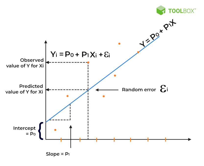
We assume the target is a straight-line function of the feature plus random noise:

\[ y_i = b_0 + b_1 x_i + \varepsilon_i \]

b₀ is the intercept (the value of y when x = 0), b₁ is the slope (how much y changes when x grows by one unit), and ε_i is the random error — everything the line cannot explain. In machine-learning notation the same model is written ŷ = w·x + b, with w the weight and b the bias.

Regression line with intercept, slope, an observed value, its predicted value on the line, and the random error between them — The anatomy of the model: each observed value of Y sits off the line by a random error ε_i; the predicted value is the point on the line. *(From Dr. Albanna's slides; the original image carries the Toolbox logo.)*

Three scatter plots: positive slope, negative slope, and no relationship — The sign of the slope tells the type of relationship: positive, negative, or none.

3. The Learning Procedure: Model, Loss, Cost

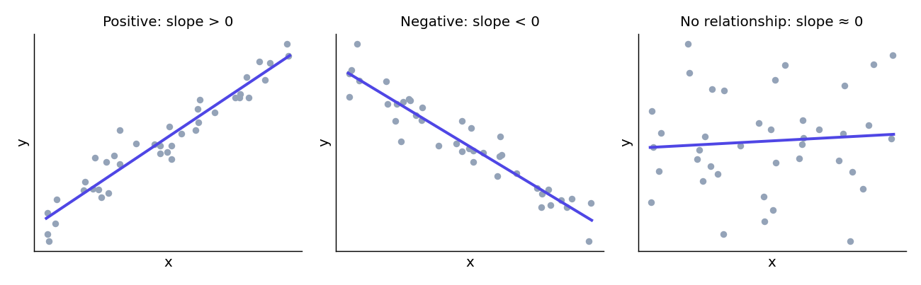
Linear regression learns to predict a real-valued target as a linear function of the inputs. Like every algorithm in this course, it follows three steps: choose a model, define a loss that says how bad the fit is, and fit the model with an optimization algorithm.

The general learning procedure, used by every model in this course: choose a model, define a loss that says how bad one prediction is, average it into a cost, then optimize. Linear regression can be solved in one step (least squares) or by repeating small updates (gradient descent, dashed loop). (After Dr. Albanna's slides and the University of Toronto CSC 311 / CSC 2515 lecture notes.)

The loss for one example is the squared error between the prediction ŷ and the true target t. Squaring makes every error positive and punishes large errors much more than small ones. The cost averages the loss over all N training examples:

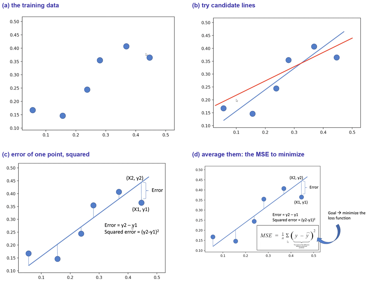
\[ \mathcal{L}(\hat y, t) = \tfrac{1}{2}(\hat y - t)^2 \qquad\qquad J(w, b) = \frac{1}{2N}\sum_{i=1}^{N}\big(w x^{(i)} + b - t^{(i)}\big)^2 \]

Four panels: the data points; two candidate lines; the error of one point and its square; the MSE formula with the goal of minimizing it — Building the loss step by step: **(a)** the training data; **(b)** many lines could fit it — which is best? **(c)** for each point, the error is the vertical gap between the point and the line, and we square it; **(d)** averaging the squared errors gives the MSE, and the best line is the one that makes it smallest. *(From Dr. Albanna's slides, adapted from the University of Toronto CSC 2515 / CSC 311 lecture notes on linear regression.)*

The ½ is only for convenience — it cancels when we differentiate. Training means finding the w and b that make J as small as possible.

4. Least Squares: The Best Line in One Step

The cost is a smooth bowl, so its minimum is where the partial derivatives with respect to both parameters are zero. Setting ∂J/∂b₁ = 0 and ∂J/∂b₀ = 0 and solving gives the least-squares estimates:

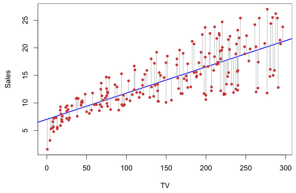
\[ b_1 = \frac{\sum_{i}(x_i - \bar x)(y_i - \bar y)}{\sum_{i}(x_i - \bar x)^2} \qquad\qquad b_0 = \bar y - b_1\,\bar x \]

Deriving the formulas, step by step

The squared error of a line. Each point’s error is the vertical gap to the line, y_i − (m x_i + b) — positive above the line, negative below. Squaring and adding them gives SE_line. (Redrawn from Dr. Albanna’s slides, which follow Khan Academy’s proof of the least-squares formulas.)

Write the line as y = m x + b (slope m, intercept b). The squared error of the line over n points is

\[ SE_{line} = \sum_{i=1}^{n}\big(y_i - (m x_i + b)\big)^2 = \big(y_1 - (m x_1 + b)\big)^2 + \dots + \big(y_n - (m x_n + b)\big)^2 \]

1

Expand every square and collect the terms

\[ \begin{aligned} SE_{line} = {} & (y_1^2 + \dots + y_n^2) - 2m(x_1y_1 + \dots + x_ny_n) - 2b(y_1 + \dots + y_n) \\ & + m^2(x_1^2 + \dots + x_n^2) + 2mb(x_1 + \dots + x_n) + nb^2 \end{aligned} \]

2

Replace each sum by n times a mean

Since (y₁² + … + y_n²) / n is the mean of y², the sum equals n·mean(y²); the same holds for the other sums:

\[ SE_{line} = n\,\overline{y^2} - 2mn\,\overline{xy} - 2bn\,\bar y + m^2 n\,\overline{x^2} + 2mbn\,\bar x + nb^2 \]

3

Find the bottom of the bowl

As a function of m and b, SE_line is a bowl: m² and b² appear with positive coefficients. Its lowest point is where the surface is flat in both directions — where both partial derivatives are zero:

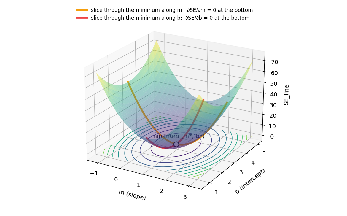
A 3-D bowl of SE over slope m and intercept b, with two slices through the minimum whose slopes are zero at the bottom — SE_line as a surface over (m, b) for a small dataset. Slicing through the minimum along m (orange) and along b (red) gives two parabolas whose slopes are zero at the bottom: `∂SE/∂m = 0` and `∂SE/∂b = 0`. *(Redrawn from Dr. Albanna’s slides, which follow Khan Academy’s proof of the least-squares formulas.)*

\[ \begin{aligned} \frac{\partial SE}{\partial m} &= -2n\,\overline{xy} + 2n\,\overline{x^2}\,m + 2bn\,\bar x = 0 \\[6pt] \frac{\partial SE}{\partial b} &= -2n\,\bar y + 2mn\,\bar x + 2bn = 0 \end{aligned} \]

4

Solve the two equations

Divide the second equation by 2n: b = ȳ − m·x̄ — so the line passes through (x̄, ȳ). Substitute this b into the first equation and solve for m:

\[ m = \frac{\overline{xy} - \bar x\,\bar y}{\overline{x^2} - \bar x^{\,2}} = \frac{\sum_i (x_i - \bar x)(y_i - \bar y)}{\sum_i (x_i - \bar x)^2} \qquad b = \bar y - m\,\bar x \]

These are exactly the formulas above (m = b₁, b = b₀).

Check with the worked example below

From the slide's sums (n = 7): Σx = 5.15, Σy = 71.403, Σxy = 49.458, Σx² = 3.9869. Means: x̄ = 0.7357, ȳ = 10.2004, mean(xy) = 7.0654, mean(x²) = 0.5696.

m = (7.0654 − 0.7357 × 10.2004) / (0.5696 − 0.7357²) = (7.0654 − 7.5046) / (0.5696 − 0.5413) = −0.4392 / 0.0283 = −15.53 — the same slope as the table method, up to the rounding of the sums.

The fitted line always passes through the point of means (x̄, ȳ). An equivalent form that avoids subtracting the means is b₁ = (nΣxy − ΣxΣy) / (nΣx² − (Σx)²).

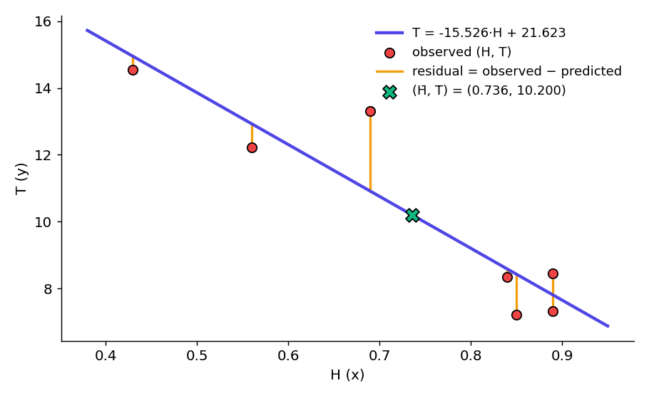
Sales against TV advertising with the least-squares line and grey residual segments — The least-squares fit for sales against TV advertising. Each grey segment is a residual; least squares chooses the line that makes the sum of their squares as small as possible. *(Textbook T1: James, Witten, Hastie & Tibshirani, An Introduction to Statistical Learning with Applications in Python, Springer 2023, Figure 3.1.)*

Worked example — fit T from H by hand

Seven observations of an input H (x) and a target T (y). Step 1: the means are H̄ = 5.15 / 7 = 0.7357 and T̄ = 71.403 / 7 = 10.2004. Step 2: fill in the deviation columns.

H (x)	T (y)	x − x̄	y − ȳ	(x − x̄)(y − ȳ)	(x − x̄)²
0.89	7.330	0.1543	−2.8704	−0.4429	0.0238
0.85	7.223	0.1143	−2.9774	−0.3403	0.0131
0.89	8.440	0.1543	−1.7604	−0.2716	0.0238
0.56	12.230	−0.1757	2.0296	−0.3566	0.0309
0.84	8.340	0.1043	−1.8604	−0.1940	0.0109
0.69	13.300	−0.0457	3.0996	−0.1417	0.0021
0.43	14.540	−0.3057	4.3396	−1.3267	0.0935
Sum				−3.0738	0.1980

Step 3: b₁ = −3.0738 / 0.1980 = −15.526. Step 4: b₀ = 10.2004 − (−15.526)(0.7357) = 21.623.

Model: T = −15.526·H + 21.623. For a new input H = 0.70 it predicts T = −15.526(0.70) + 21.623 = 10.75.

Download this calculation as a spreadsheet

The seven (H, T) points, the fitted line T = -15.526 H + 21.623, and the residuals — The worked example plotted: the fitted line, each residual, and the point of means it passes through.

5. Gradient Descent

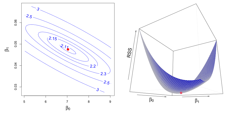
Least squares has a closed-form answer only because the model is so simple. Gradient descent is a second way to minimize the cost that works for almost every model in machine learning, including neural networks. It is iterative: start from any weights (e.g. all zeros) and repeatedly step in the direction of steepest descent — opposite to the gradient — until the cost stops falling.

\[ w \leftarrow w - \eta\,\frac{\partial J}{\partial w} = w - \eta\,\frac{1}{N}\sum_{i}(\hat y^{(i)} - t^{(i)})\,x^{(i)} \qquad b \leftarrow b - \eta\,\frac{1}{N}\sum_{i}(\hat y^{(i)} - t^{(i)}) \]

η (eta) is the learning rate, the size of each step. Both parameters are updated at the same time, using the gradient computed with the old values.

Contour plot and 3-D surface of the residual sum of squares over the intercept and slope, with the minimum marked — The cost (RSS) as a surface over the two parameters: a single bowl with one minimum (red dot). Gradient descent walks downhill on this surface; least squares jumps straight to the bottom. *(Textbook T1: James et al., ISLP, Figure 3.2.)*

Gradient descent steps on a parabola for a small, a good and a large learning rate — The learning rate decides everything: too small crawls, a good value reaches the minimum in a few steps, too large overshoots back and forth (and if larger still, diverges).

Worked example — one gradient-descent step by hand

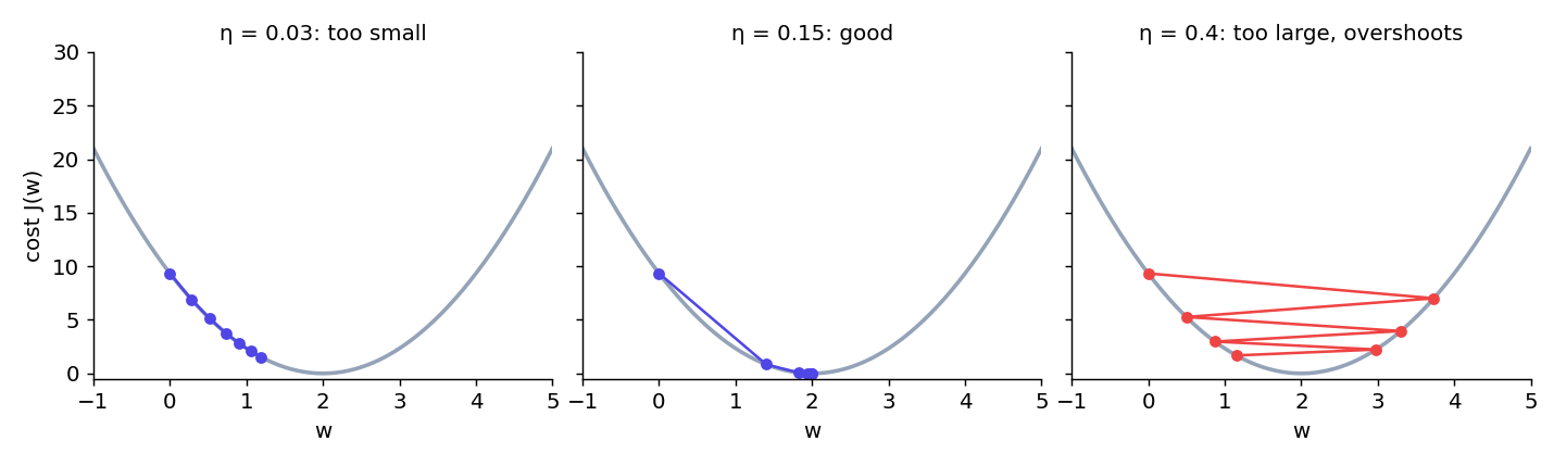
Data: x = [1, 2, 3], t = [2, 4, 6] (the true answer is w = 2, b = 0). Start at w = 0, b = 0 with η = 0.1.

Predict: ŷ = [0, 0, 0]; errors ŷ − t = [−2, −4, −6]. Cost J = (4 + 16 + 36) / (2·3) = 9.33.

Gradients: ∂J/∂w = (−2·1 − 4·2 − 6·3) / 3 = −28/3 = −9.33; ∂J/∂b = (−2 − 4 − 6) / 3 = −4.

Update: w = 0 − 0.1(−9.33) = 0.933; b = 0 − 0.1(−4) = 0.4. New cost J = 1.88 — down from 9.33. One more step gives w = 1.351, b = 0.573, J = 0.40; after a few hundred steps w → 2, b → 0.

	Least squares (closed form)	Gradient descent
How	Solve ∂J = 0 directly	Repeat small downhill steps
Hyperparameters	None	Learning rate, number of iterations
Large data / many features	Slow (matrix inverse)	Scales well (and mini-batch versions scale further)
Other models	Only linear regression	Logistic regression, neural networks, …

Scale your features

When features have very different ranges, the cost bowl becomes a long narrow valley and gradient descent zig-zags. Standardizing the features first (Module 2) makes it converge much faster.

6. Multiple Linear Regression

With p features the line becomes a plane (or a hyperplane in more dimensions):

\[ \hat y = w_1 x_1 + w_2 x_2 + \dots + w_p x_p + b = \mathbf{w}^\top \mathbf{x} + b \]

Each coefficient w_j is the change in the prediction when x_j grows by one unit while all other features stay fixed. Stacking the N training examples as the rows of a matrix X (with a column of 1s for the bias), least squares has a matrix solution, the normal equation:

\[ \mathbf{w} = (X^\top X)^{-1} X^\top \mathbf{y} \]

Points in 3-D above and below a fitted regression plane over two features — With two features, least squares fits the plane that minimizes the sum of squared vertical distances to the points. *(Textbook T1: James et al., ISLP, Figure 3.4.)*

Worked example — using a fitted model

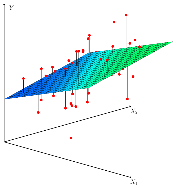
A house-price model: price = 50 + 120·size + 15·rooms − 2·age (price in $1000s, size in 100 m², age in years). A 150 m² house with 4 rooms, 10 years old: 50 + 120(1.5) + 15(4) − 2(10) = 50 + 180 + 60 − 20 = 270 → $270,000. Reading the coefficients: one extra room adds $15,000 for a house of the same size and age; each year of age subtracts $2,000.

7. How Good Is the Fit?

Three families of metrics evaluate a regression model (Module 5 covers them in full):

\[ \text{MAE} = \frac{1}{n}\sum|y_i - \hat y_i| \qquad \text{MSE} = \frac{1}{n}\sum(y_i - \hat y_i)^2 \qquad \text{RMSE} = \sqrt{\text{MSE}} \]

MAE — the average size of an error, in the units of y. Robust to outliers.
MSE — squares the errors, so large errors weigh much more. Units are squared.
RMSE — back in the units of y; the typical size of an error.

R²: the proportion of variance explained

Split each point's distance from the mean into a part the line explains and a part it does not. Summed over all points, SS_total = SS_regression + SS_residual, and

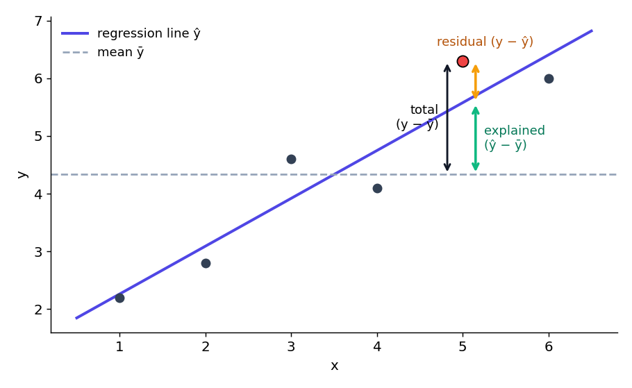
\[ R^2 = \frac{SS_{reg}}{SS_{total}} = 1 - \frac{SS_{res}}{SS_{total}} = 1 - \frac{\sum(y_i - \hat y_i)^2}{\sum(y_i - \bar y)^2} \]

One point's distance from the mean split into an explained part and a residual part — For one point: total = explained + residual. R² is the explained share of the total, summed over all points. *(After Dr. Albanna's slides.)*

R² runs from 0 (the line is no better than predicting the mean) to 1 (a perfect fit). It is positive even when the slope is negative — it measures fit, not direction.

Adjusted R²

Plain R² never goes down when you add a feature, even a useless one. Adjusted R² charges a penalty for every extra feature (n = observations, k = features):

\[ R^2_{adj} = 1 - (1 - R^2)\,\frac{n - 1}{n - k - 1} \]

Worked example — all the metrics

Example from Statistics How To, “Mean Squared Error”.

Points (43, 41), (44, 45), (45, 49), (46, 47), (47, 44); least squares gives ŷ = 9.2 + 0.8x.

x	y	ŷ	error y − ŷ	error²	(y − ȳ)²
43	41	43.6	−2.6	6.76	17.64
44	45	44.4	0.6	0.36	0.04
45	49	45.2	3.8	14.44	14.44
46	47	46.0	1.0	1.00	3.24
47	44	46.8	−2.8	7.84	1.44
Sum (ȳ = 45.2)				30.40	36.80

MSE = 30.4 / 5 = 6.08; RMSE = √6.08 = 2.47; MAE = (2.6 + 0.6 + 3.8 + 1.0 + 2.8) / 5 = 2.16; R² = 1 − 30.4 / 36.8 = 0.174; R²_adj = 1 − (0.826)(4 / 3) = −0.10. A negative adjusted R² is a warning: with only 5 points, x explains almost nothing about y.

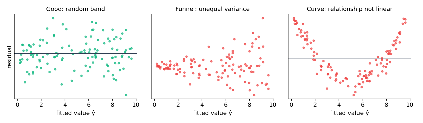
8. Assumptions of Linear Regression

The least-squares estimates are trustworthy only when the data meets a few assumptions. Check them with a residual plot (residual against prediction):

Assumption	Meaning	Symptom when it fails
Linearity	The relationship between x and y is a straight line	Residuals form a curve
Independence	Observations (and their errors) do not depend on each other	Patterns over time in the residuals (autocorrelation)
Normality	Errors are normally distributed around the line	Skewed histogram of residuals
Equal variance (homoscedasticity)	The spread of y is the same at every x	Residuals fan out in a funnel
No multicollinearity (multiple regression)	Features are not strongly correlated with each other	Unstable coefficients with unexpected signs

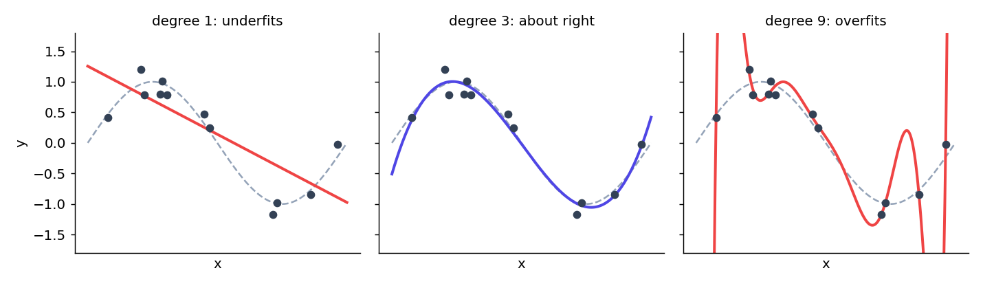
Three residual plots: a random band, a funnel, and a curve — What to look for: a structureless band is good; a funnel means unequal variance; a curve means the relationship is not linear (try polynomial features, Section 9).

9. Polynomial Regression and Overfitting

When the relationship is curved, we can still use linear regression: create new features x², x³, … and fit a linear model on them. The model stays linear in its weights, so least squares and gradient descent work unchanged:

\[ \hat y = w_1 x + w_2 x^2 + \dots + w_M x^M + b \]

Polynomials of degree 1, 3 and 9 fit to the same 12 points — Twelve noisy points from a sine curve (dashed). Degree 1 underfits, degree 3 captures the shape, degree 9 passes through the points but swings wildly between them — it fits the noise.

Training error keeps falling while test error is U-shaped as the number of parameters grows — As the number of parameters grows, training error keeps falling but test error falls and then rises. *(From Dr. Albanna's slides; figure from the University of Toronto CSC 2515 lecture notes, “Linear Models”.)*

How to avoid overfitting

Use a lower-degree polynomial (fewer parameters) — but too low underfits.
Get more training data — often expensive or impossible.
Regularize: keep all the features but penalize large weights. A sign of overfitting is huge coefficients that cancel each other out.

10. Regularization: Ridge and Lasso

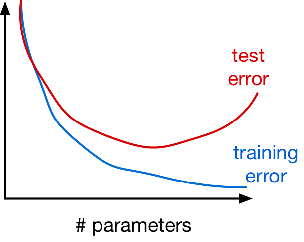
Regularization adds a penalty on the size of the weights to the cost. The hyperparameter α (also written λ) sets how strong the penalty is.

\[ \begin{aligned} \text{Ridge (L2):}\quad J &= \sum_i (y_i - \hat y_i)^2 + \alpha \sum_j w_j^2 \\[6pt] \text{Lasso (L1):}\quad J &= \sum_i (y_i - \hat y_i)^2 + \alpha \sum_j |w_j| \end{aligned} \]

	Ridge (L2)	Lasso (L1)
Penalty	Sum of squared weights	Sum of absolute weights
Effect	Shrinks all weights toward 0, but none to exactly 0	Shrinks and sets some weights exactly to 0
Use it when	Many features all contribute a little; multicollinearity	You suspect only a few features matter — it does feature selection

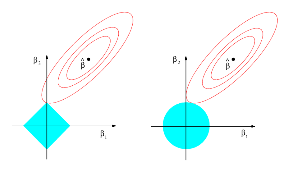
Lasso diamond and ridge circle constraint regions touched by elliptical cost contours — Why Lasso zeroes weights: the red ellipses are contours of the cost, centred at the unregularized solution β̂. The answer is where they first touch the constraint region — the Lasso **diamond** (left) has corners on the axes, so the touch often happens at `β₁ = 0`; the Ridge **circle** (right) has no corners. *(Textbook T1: James et al., ISLP, Figure 6.7.)*

Choosing α

α = 0 gives ordinary least squares (risk of overfitting); a very large α pushes all weights to 0 (underfitting). Split the training data into train and validation sets, train one model per candidate α (e.g. 0.001, 0.01, 0.1, 1, 10, 100), and keep the one with the lowest validation error — or use cross-validation. Report the final score on the untouched test set. Standardize the features first, so the penalty treats them all equally.

Worked example — the penalty terms

Weights w = (3, −2, 0.5), sum of squared errors 40, α = 2. Ridge: 40 + 2(9 + 4 + 0.25) = 40 + 26.5 = 66.5. Lasso: 40 + 2(3 + 2 + 0.5) = 40 + 11 = 51. Training then trades a little extra error for smaller weights.

Python Lab

Run this in Google Colab. Part 1 reproduces the worked example three ways — by the formula, with scikit-learn, and with gradient descent written from scratch — and all three give the same line. Part 2 fits multiple, Ridge and Lasso regression on the built-in diabetes dataset (10 features).

import numpy as np
from sklearn.linear_model import LinearRegression, Ridge, Lasso
from sklearn.datasets import load_diabetes
from sklearn.model_selection import train_test_split
from sklearn.metrics import mean_absolute_error, mean_squared_error, r2_score

# ---- Part 1: the worked example ----
H = np.array([0.89, 0.85, 0.89, 0.56, 0.84, 0.69, 0.43])
T = np.array([7.33, 7.223, 8.44, 12.23, 8.34, 13.3, 14.54])

# (a) least-squares formulas
b = ((H - H.mean()) * (T - T.mean())).sum() / ((H - H.mean()) ** 2).sum()
a = T.mean() - b * H.mean()
print(f"least squares by hand: T = {b:.3f}*H + {a:.3f}")

# (b) scikit-learn (expects a 2-D feature matrix)
lr = LinearRegression().fit(H.reshape(-1, 1), T)
print(f"scikit-learn:          T = {lr.coef_[0]:.3f}*H + {lr.intercept_:.3f}")

# (c) gradient descent from scratch
w, c, eta = 0.0, 0.0, 1.0
for step in range(20000):
    err = (w * H + c) - T                 # prediction minus target
    w -= eta * (err * H).mean()           # dJ/dw
    c -= eta * err.mean()                 # dJ/db
print(f"gradient descent:      T = {w:.3f}*H + {c:.3f}")
# all three print  T = -15.526*H + 21.623

# ---- Part 2: multiple regression, Ridge and Lasso ----
X, y = load_diabetes(return_X_y=True)          # 442 patients, 10 (already scaled) features
X_tr, X_te, y_tr, y_te = train_test_split(X, y, test_size=0.25, random_state=0)
for name, model in [("Linear", LinearRegression()), ("Ridge a=0.1", Ridge(alpha=0.1)), ("Lasso a=1", Lasso(alpha=1.0))]:
    model.fit(X_tr, y_tr)
    p = model.predict(X_te)
    print(f"{name:12s} MAE={mean_absolute_error(y_te, p):5.1f}  RMSE={mean_squared_error(y_te, p) ** 0.5:5.1f}  "
          f"R2={r2_score(y_te, p):.3f}  zero coefficients={np.sum(model.coef_ == 0)}")
# Linear       MAE= 45.1  RMSE= 56.4  R2=0.359  zero coefficients=0
# Ridge a=0.1  MAE= 44.6  RMSE= 56.0  R2=0.369  zero coefficients=0
# Lasso a=1    MAE= 48.3  RMSE= 59.9  R2=0.278  zero coefficients=8

Try it

Lasso with α = 1 kept only 2 of the 10 features — too strong a penalty. Try α = 0.01, 0.1, 0.5: how many coefficients are zero each time, and which α gives the best test R²? In part 1, set eta = 5 and watch gradient descent diverge.

More examples from class (house size vs. price, California housing, study hours vs. exam score) are in the notebooks: LR Part 1 (.ipynb) LR Part 2 (.ipynb)

Textbook Reading

From the course syllabus

T1 James et al. — ISLP, Ch. 3 Linear Regression (§3.1 simple, §3.2 multiple, §3.3.2 extensions of the linear model, including polynomial regression) and §6.2 Shrinkage Methods (ridge and lasso).
T2 Murphy — Probabilistic Machine Learning, Ch. 11 Linear Regression (§11.2 least squares, §11.3 ridge, §11.4 lasso) and §8.2 first-order methods (gradient descent).

Both books are free to read online from their authors: statlearning.com (T1) and probml.github.io (T2).

Exercises

1

GDP and vehicle sales (from class)

X = GDP, Y = passenger-vehicle sales (in 0.1 millions): 2011 (6.2, 26.3), 2012 (6.5, 26.65), 2013 (5.48, 25.03), 2014 (6.54, 26.01), 2015 (7.18, 27.9), 2016 (7.93, 30.47). Find (1) the regression equation, (2) MSE and RMSE, (3) MAE, (4) R², (5) the predicted sales when GDP = 7.23.

Means: x̄ = 6.638, ȳ = 27.06. Σ(x−x̄)(y−ȳ) = 7.704, Σ(x−x̄)² = 3.524. (1) b₁ = 7.704 / 3.524 = 2.186, b₀ = 27.06 − 2.186(6.638) = 12.549 → Y = 12.549 + 2.186X. Predictions: 26.10, 26.76, 24.53, 26.85, 28.24, 29.88; errors: 0.198, −0.108, 0.502, −0.835, −0.344, 0.587. (2) MSE = 0.244, RMSE = 0.494. (3) MAE = 0.429. (4) R² = 0.920 — GDP explains 92% of the variation in sales. (5) 12.549 + 2.186(7.23) = 28.35, i.e. about 2.84 million vehicles.

2

Least squares by hand

Hours studied x = [1, 2, 3, 4, 5], exam score y = [52, 55, 61, 64, 68]. Find the least-squares line and predict the score for 6 hours.

x̄ = 3, ȳ = 60. Deviations x: −2, −1, 0, 1, 2; y: −8, −5, 1, 4, 8. Σ(x−x̄)(y−ȳ) = 16 + 5 + 0 + 4 + 16 = 41; Σ(x−x̄)² = 10. b₁ = 4.1, b₀ = 60 − 4.1(3) = 47.7. Line: ŷ = 47.7 + 4.1x; for 6 hours: 47.7 + 24.6 = 72.3.

3

A gradient-descent step

Data x = [1, 2], t = [3, 5]. Start at w = 1, b = 0 with η = 0.1. Compute the cost (with ½N), both gradients, the updated w and b, and the new cost.

ŷ = [1, 2]; errors ŷ − t = [−2, −3]. J = (4 + 9) / 4 = 3.25. ∂J/∂w = (−2·1 − 3·2) / 2 = −4; ∂J/∂b = (−2 − 3) / 2 = −2.5. Update: w = 1 + 0.4 = 1.4, b = 0 + 0.25 = 0.25. New ŷ = [1.65, 3.05]; errors [−1.35, −1.95]; J = (1.8225 + 3.8025) / 4 = 1.41 — the cost fell from 3.25 to 1.41.

4

Adjusted R²

Model A uses 2 features and has R² = 0.80; model B adds 8 more features and reaches R² = 0.82. Both were fit on n = 30 observations. Compute adjusted R² for each. Which model do you prefer?

A: 1 − 0.20 × 29/27 = 1 − 0.2148 = 0.785. B: 1 − 0.18 × 29/19 = 1 − 0.2747 = 0.725. Prefer A: the 8 extra features raised R² only slightly, and adjusted R² shows they do not pay for their complexity.

5

Read the residual plot

After fitting income against years of experience, the residuals are small for junior staff and grow steadily larger for senior staff. Which assumption is violated, and what could you do?

The residuals fan out like a funnel: equal variance (homoscedasticity) is violated. Remedies: transform the target (e.g. model log(income)), use weighted least squares, or report robust standard errors.

6

Ridge or Lasso?

(a) You have 500 genes and believe only about 10 affect a disease. (b) You have 20 economic indicators, many strongly correlated, all believed to matter a little. (c) What happens to both models as α → 0, and as α → ∞?

(a) Lasso — it sets the irrelevant genes' weights to exactly 0, selecting the few that matter. (b) Ridge — it shrinks correlated weights together and keeps them all. (c) As α → 0 both become ordinary least squares (may overfit); as α → ∞ all weights go to 0 and the model predicts a constant (underfits).

Recap & Where Next

You now know

Linear regression predicts a number with ŷ = w·x + b; training minimizes the mean squared error.
Least squares gives the answer in one step: b₁ = Σ(x−x̄)(y−ȳ) / Σ(x−x̄)², b₀ = ȳ − b₁x̄; the normal equation does the same for many features.
Gradient descent reaches the same answer by repeated steps w ← w − η·∂J/∂w, and works for models with no closed form.
MAE, MSE, RMSE, R² and adjusted R² measure the fit; residual plots check the assumptions.
Polynomial features fit curves but invite overfitting; Ridge shrinks weights, Lasso also zeroes them; tune α on validation data.

Regression predicts numbers. What if the answer is yes or no? Module 4 bends the straight line through a sigmoid to get logistic regression, our first classifier.