Our first classifier: bend a straight line through the sigmoid to get the probability of a yes/no outcome, train it by maximum likelihood, and choose where to draw the line between yes and no.
Module 4 · Weeks 4–5 · Lecture notes by Dr. Abdulkarim Albanna
Core Supervised · Classification ~65 minp = σ(w·x + b)Prerequisite: Module 3. Logistic regression reuses the linear model w·x + b and gradient descent from linear regression.
Often we care about an input–output relationship, just as in regression, but the output is discrete, not continuous: spam or not, sick or healthy, pass or fail. Guessing the class from the inputs is classification. In binary classification the target is t ∈ {0, 1}; examples with t = 1 are the positive examples and those with t = 0 the negative ones.
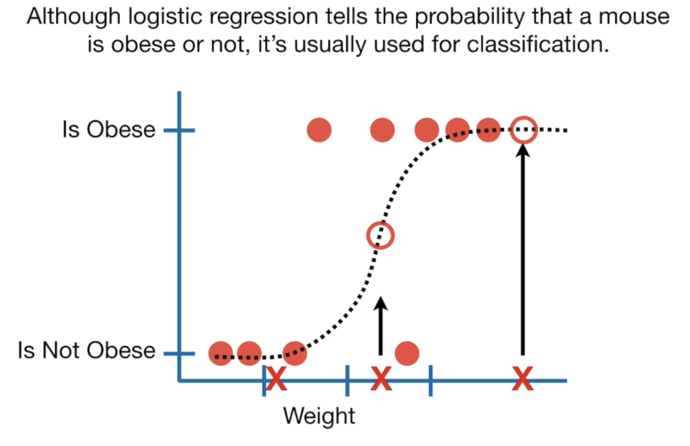
Rather than guessing the class directly, logistic regression models the probability P(Y = 1 | X = x) as a function of x, and estimates the unknown parameters by maximum likelihood. Despite its name it is a classification method; “regression” refers to the linear model it fits inside.
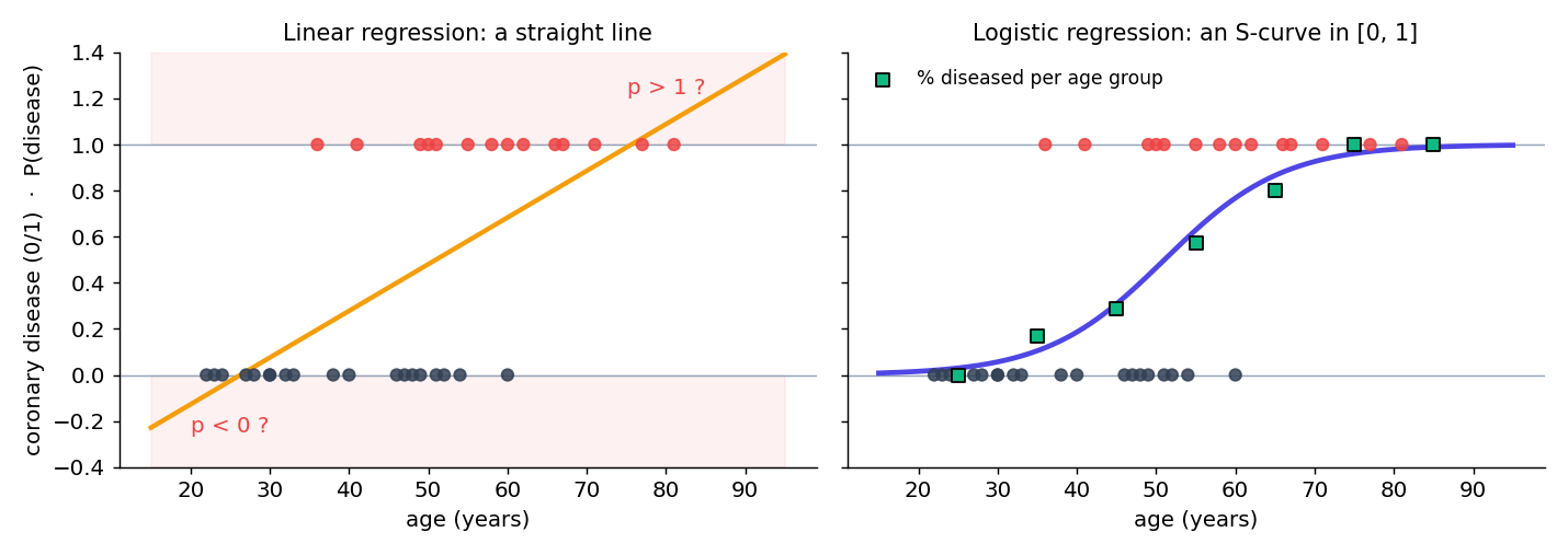
33 adults, their age, and whether they show signs of coronary heart disease (CD = 1) or not (CD = 0). 14 have the disease. The mean age is 38.6 years in the healthy group and about 59 years in the diseased group — so age matters. Grouping by age makes the pattern clear:
| Age group | 20–29 | 30–39 | 40–49 | 50–59 | 60–69 | 70–79 | 80–89 |
|---|---|---|---|---|---|---|---|
| People in group | 5 | 6 | 7 | 7 | 5 | 2 | 1 |
| Diseased | 0 | 1 | 2 | 4 | 4 | 2 | 1 |
| % diseased | 0% | 17% | 29% | 57% | 80% | 100% | 100% |
The percentage climbs along an S-shape from 0 to 100%. That S is what logistic regression fits.
| Linear regression | Logistic regression | |
|---|---|---|
| Predicts | A continuous value | The probability of a class |
| Shape | Straight line | S-shaped (sigmoid) curve |
| Task | Regression | Classification |
| Fitted by | Least squares / gradient descent | Maximum likelihood (gradient descent) |
| Fit measured by | MSE, R² | Log-loss (−2 log-likelihood), accuracy, precision, recall |
| Type | Target | Examples |
|---|---|---|
| Binomial (binary) | Two categories | Yes / No, Pass / Fail, Spam / Not spam — the most common, and the focus of this module |
| Multinomial | Three or more unordered categories | Cat / Dog / Sheep; which product a customer buys (uses softmax) |
| Ordinal | Three or more ordered categories | Low / Medium / High; a 1–5 star rating |
The sigmoid (or logistic) function takes any real number and squashes it into the range (0, 1), drawing an S-shaped curve:
σ(z) → 1 as z → +∞, and σ(z) → 0 as z → −∞; it is always strictly between 0 and 1.σ(0) = 0.5; the curve is symmetric: σ(−z) = 1 − σ(z).σ'(z) = σ(z)(1 − σ(z)) — handy for gradient descent.σ(5x) is steeper, and σ(5x − 10) is steeper and centred at x = 2.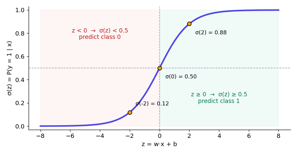
Logistic regression takes the linear model from Module 3, z = w·x + b = w1x1 + … + wnxn + b, whose output is any real number, and feeds it through the sigmoid to get a probability:
Why the sigmoid? Because it is the inverse of the logit, the function that turns a probability into a number a straight line can model.
odds = p / (1 − p). If P(Y = 1) = 0.8, the odds are 0.8 / 0.2 = 4 (“4 to 1”).logit(p) = log(p / (1 − p)). It maps a probability in (0, 1) onto the whole real line (−∞, +∞).Logistic regression assumes the log-odds are linear in x. Solving for p gives back the sigmoid:
b is the log-odds when all features are 0.wj is the change in log-odds when xj grows by one unit (all else fixed).ewj is the odds ratio: the odds are multiplied by ewj for each one-unit increase in xj.A model of survival for patients exposed to a disease: log(P / (1 − P)) = 1.8158 − 0.0665·Age.
Newborn (Age = 0): log-odds = 1.8158 → odds = e1.8158 = 6.15 → P = 6.15 / (1 + 6.15) = 0.86.
Age 25: log-odds = 1.8158 − 0.0665(25) = 0.1533 → odds = e0.1533 = 1.17 → P = 1.17 / 2.17 = 0.54.
The odds ratio per year is e−0.0665 = 0.936: each extra year multiplies the odds of survival by 0.936, about a 6.4% drop.
Logistic regression has no residuals in the least-squares sense, so we cannot use least squares or R². Instead it uses maximum likelihood estimation (MLE): choose the parameters that make the observed labels as probable as possible.
For each example the model gives pi = P(yi = 1 | xi). The probability it assigns to the label actually observed is pi if yi = 1 and 1 − pi if yi = 0. Assuming independent examples, the likelihood of the whole dataset is the product, and since log is increasing we maximize the easier log-likelihood (a sum):
Because every pi < 1, ℓ is negative. Maximizing ℓ is the same as minimizing −2ℓ (the deviance) or the average log-loss (binary cross-entropy):
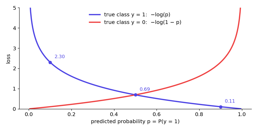
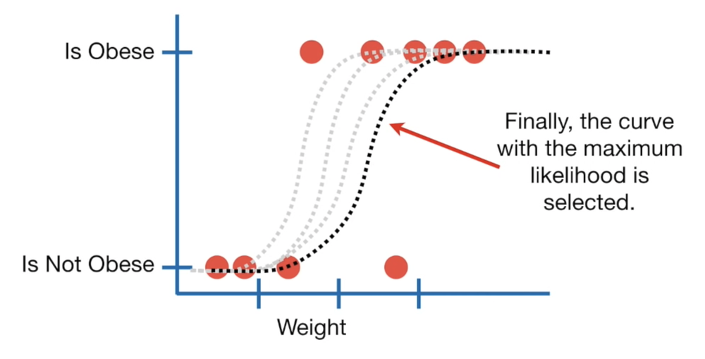
There is no closed-form solution, so the parameters are found iteratively: start from zeros, compute the log-likelihood, adjust the coefficients, and repeat until it stops improving. The gradient of the log-loss has the same shape as in linear regression — only ŷ is now a sigmoid:
At the optimum, Σ(yi − pi)xij = 0 for every feature — the condition the maximum-likelihood estimates solve.
Data x = [1, 2], y = [0, 1]; start at w = 0, b = 0, η = 1. Then z = [0, 0], p = [0.5, 0.5], and the log-loss is −(log 0.5 + log 0.5) / 2 = 0.693.
Gradients: ∂J/∂w = ((0.5 − 0)·1 + (0.5 − 1)·2) / 2 = −0.25; ∂J/∂b = ((0.5 − 0) + (0.5 − 1)) / 2 = 0. Update: w = 0.25, b = 0.
Now p = [σ(0.25), σ(0.5)] = [0.562, 0.622] and the log-loss is −(log 0.438 + log 0.622) / 2 = 0.650 — lower than 0.693.
Four observations from a binomial distribution with n = 3 trials each: (1, 3, 2, 2) successes. Find the success probability θ.
Likelihood: L(θ) = C(3,1)θ(1−θ)² · C(3,3)θ³ · C(3,2)θ²(1−θ) · C(3,2)θ²(1−θ) = 27θ8(1−θ)4.
Log-likelihood: ℓ(θ) = ln 27 + 8 ln θ + 4 ln(1−θ). Derivative: 8/θ − 4/(1−θ) = 0 → 8(1−θ) = 4θ → θ̂ = 8/12 = 2/3 — total successes over total trials, as intuition says.
To turn a probability into a class we pick a threshold t: predict class 1 if p ≥ t, else class 0. The default is t = 0.5. Since σ(z) ≥ 0.5 exactly when z ≥ 0, the default rule is simply w·x + b ≥ 0. The set of points where w·x + b = 0 is the decision boundary — a point for one feature, a line for two, a plane for three: logistic regression is a linear classifier.
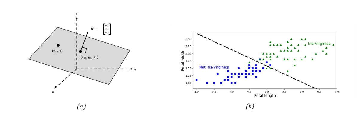
w·x + b = 0 is a plane whose normal is w. (b) A logistic regression on two iris features: the dashed line separates Iris-Virginica from the other flowers. (Textbook T2: K. P. Murphy, Probabilistic Machine Learning: An Introduction, MIT Press 2022, Figure 10.1; CC BY-NC-ND.)Moving the threshold trades one kind of error for another. A low threshold flags more positives: it catches more true cases (higher recall) but raises more false alarms. A high threshold is more cautious: fewer false alarms (higher precision) but more missed cases. In medicine, missing a sick patient is usually worse, so the threshold is set below 0.5. Module 5 measures these trade-offs with precision, recall and the ROC curve.
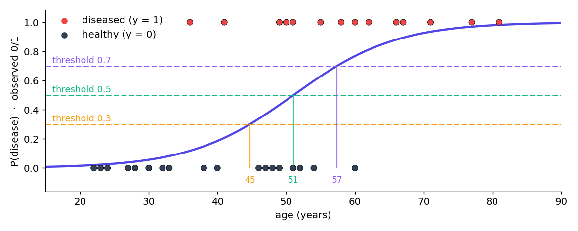
| Threshold | Cut-off age | True positives | False positives | Missed (false negatives) | True negatives | Accuracy |
|---|---|---|---|---|---|---|
| 0.3 | ≥ 45 | 12 | 8 | 2 | 11 | 69.7% |
| 0.5 | ≥ 51 | 9 | 3 | 5 | 16 | 75.8% |
| 0.7 | ≥ 57 | 8 | 1 | 6 | 18 | 78.8% |
The threshold with the best accuracy (0.7) misses 6 of the 14 sick patients; the 0.3 threshold misses only 2. Which one is “best” depends on the cost of each kind of mistake, not on accuracy alone.
Fitting logistic regression by maximum likelihood to the 33 patients from Section 1 gives:
Age 60: z = −6.820 + 0.1336(60) = 1.197 → p = 1 / (1 + e−1.197) = 0.768 → 77% chance of disease; at t = 0.5, predict disease.
Age 40: z = −6.820 + 5.344 = −1.475 → p = 0.186 → predict healthy.
Odds ratio: e0.1336 = 1.143 — every extra year multiplies the odds of disease by 1.143 (+14%); ten years multiply them by e1.336 = 3.80.
Decision boundary: z = 0 → Age = 6.820 / 0.1336 = 51.0 years.
Fit: log-likelihood −14.20, so −2LL = 28.40; average log-loss 0.430.
| Age | 30 | 40 | 50 | 60 | 70 |
|---|---|---|---|---|---|
| log-odds z | −2.81 | −1.48 | −0.14 | 1.20 | 2.53 |
| odds ez | 0.06 | 0.23 | 0.87 | 3.31 | 12.6 |
| P(disease) | 0.057 | 0.186 | 0.465 | 0.768 | 0.926 |
With several features — continuous, binary, ordinal or (one-hot encoded) nominal — the log-odds are a linear combination of all of them:
Each wj is now the increase in log-odds for a one-unit increase in xj with all other features held constant — its association with the outcome, adjusted for the others.
Extending the survival model with Gender (0 = male, 1 = female): log(P / (1 − P)) = 1.8158 − 0.0665·Age + 1.5972·Gender.
Male model (Gender = 0): 1.8158 − 0.0665·Age. Female model (Gender = 1): (1.8158 + 1.5972) − 0.0665·Age = 3.4130 − 0.0665·Age.
At age 25: male z = 0.153 → P = 0.54; female z = 1.751 → P = 0.85. The odds ratio for being female is e1.5972 = 4.94: at any age, a woman's odds of survival are about 4.9 times a man's.
Run this in Google Colab. It fits the coronary-disease model with scikit-learn, prints the probabilities and the effect of the threshold, then re-fits the same model with gradient descent written from scratch.
Remove penalty=None. scikit-learn then applies L2 regularization by default (Module 3): how do the coefficient and the probabilities change? Then try thresholds 0.4 and 0.6 and fill in the table.
The class notebook adds a 2-D example with a plotted decision boundary, the sigmoid and log-loss curves, and every classification metric: Logistic regression example (.ipynb)
Both books are free to read online from their authors: statlearning.com (T1) and probml.github.io (T2).
A model has w = 2, b = −3. Compute P(y = 1) for x = 1 and x = 2, and the class at threshold 0.5. Where is the decision boundary?
x = 1: z = 2 − 3 = −1, p = 1 / (1 + e) = 0.269 → class 0. x = 2: z = 4 − 3 = 1, p = 0.731 → class 1. Boundary: 2x − 3 = 0 → x = 1.5.
(a) Convert p = 0.75 to odds and log-odds. (b) Convert log-odds −1 to a probability. (c) What probability has log-odds 0?
(a) odds = 0.75 / 0.25 = 3; log-odds = ln 3 = 1.099. (b) p = 1 / (1 + e1) = 0.269. (c) p = 0.5 (odds = 1).
In the coronary-disease model the age coefficient is 0.1336. What is the odds ratio for one year, and for ten years? Explain each in one sentence.
One year: e0.1336 = 1.143 — each extra year multiplies the odds of disease by 1.143 (14% higher). Ten years: e1.336 = 3.80 — someone ten years older has about 3.8 times the odds. Note it is the odds that are multiplied, not the probability.
Three examples with true labels y = [1, 0, 0] and predicted probabilities p = [0.9, 0.3, 0.6]. Compute each loss and the average. Which prediction is the worst?
Example 1 (y = 1): −ln 0.9 = 0.105. Example 2 (y = 0): −ln(1 − 0.3) = 0.357. Example 3 (y = 0): −ln(1 − 0.6) = 0.916. Average = 1.378 / 3 = 0.459. The third is worst: it gave 60% to the wrong class.
Eight predicted probabilities with their true labels: 0.92 (1), 0.75 (1), 0.58 (0), 0.45 (1), 0.40 (0), 0.22 (1), 0.15 (0), 0.08 (0). Count TP, FP, FN and TN at threshold 0.5 and at 0.3. Which threshold would you use to screen for a serious disease?
t = 0.5: predicted 1 = {0.92, 0.75, 0.58} → TP = 2, FP = 1; FN = 2 (0.45, 0.22), TN = 3. t = 0.3: 0.45 and 0.40 also become 1 → TP = 3, FP = 2, FN = 1 (0.22), TN = 2. For screening a serious disease use 0.3: it misses fewer sick patients, at the cost of one more false alarm, which a follow-up test can resolve.
A coin lands heads 7 times in 10 tosses. Write the log-likelihood of θ = P(heads), differentiate, and find the maximum-likelihood estimate.
L(θ) = θ7(1 − θ)3, so ℓ(θ) = 7 ln θ + 3 ln(1 − θ). dℓ/dθ = 7/θ − 3/(1 − θ) = 0 → 7(1 − θ) = 3θ → θ̂ = 7/10 = 0.7.
P(y = 1 | x) = σ(w·x + b), a probability between 0 and 1.log(p / (1 − p)) are linear in x; ew is the odds ratio for a one-unit increase.(p − y)x.w·x + b = 0 is linear; moving the threshold trades missed cases for false alarms.Accuracy alone hid the missed patients in Section 7. Module 5 gives us the full toolkit: the confusion matrix, precision, recall, F1, ROC curves and AUC — plus the regression metrics.