Performance Measures - Machine Learning

What You'll Learn

How to build and read a confusion matrix: TP, FN, FP, TN, P, N
Accuracy and error rate, and why accuracy fails on imbalanced data
Precision, recall, F1 and Fβ, and the four rates TPR, FNR, TNR (specificity), FPR
Metrics for multi-class problems: per-class scores, macro and micro averages
The ROC curve and the AUC, built by moving the decision threshold
Regression metrics: MAE, MSE, RMSE, R², adjusted R² — and how to choose the right metric

Prerequisites: Modules 1, 3 and 4. Every number in this module is computed on test data — data the model did not train on (holdout or cross-validation, Modules 1–2).

1. Evaluating a Model

After training we need to answer three questions: How accurate is the model on new data? Which of several models is best? Is it good enough to use? The answers come from evaluation metrics computed on a validation or test set of labelled examples — never on the training set, which would reward overfitting.

Problem type	Metrics in this module
Classification	Confusion matrix, accuracy, error rate, precision, recall (sensitivity), specificity, F1, Fβ, ROC curve, AUC
Regression	MAE, MSE, RMSE, R², adjusted R²

To estimate them reliably use the holdout method or k-fold cross-validation, and compare classifiers with ROC curves (Section 9).

2. The Confusion Matrix

A confusion matrix compares the predicted classes with the actual ones. Rows are the actual class, columns the predicted class; entry CM_i,j counts the examples of class i that the classifier labelled as class j. A good classifier puts almost everything on the diagonal.

The four outcomes, with an example

A test classifies people as pregnant (positive) or not pregnant (negative):

True Positive (TP) — actually pregnant, classified pregnant.
True Negative (TN) — actually not pregnant, classified not pregnant.
False Positive (FP) — actually not pregnant, classified pregnant (a false alarm, type I error).
False Negative (FN) — actually pregnant, classified not pregnant (a miss, type II error).

Totals: P = TP + FN actual positives, N = FP + TN actual negatives; P' = TP + FP predicted positives, N' = FN + TN predicted negatives.

How to read a confusion matrix, with the cat example (Example 1). Rows are the truth, columns are the prediction. Green cells are correct, amber cells are errors. Recall reads across the actual-positive row; precision reads down the predicted-positive column; accuracy is the diagonal.

Left: blue and red points split by a line. Right: the confusion matrix 6 true positives, 1 false negative, 2 false positives, 5 true negatives — A model is trained so the region above the line is positive (blue) and below is negative (red). Counting the points gives TP = 6, FN = 1, FP = 2, TN = 5. We will use these 14 points throughout. *(From Dr. Albanna's slides; image from Udacity’s machine-learning course, Evaluation Metrics lesson (Luis Serrano).)*

3. Accuracy and Error Rate

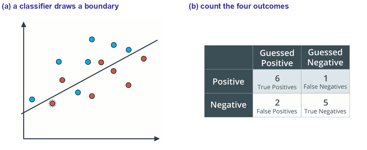
Accuracy (recognition rate) is the fraction of all examples classified correctly; the error rate is the rest:

\[ \begin{aligned} \text{Accuracy} &= \frac{TP + TN}{TP + TN + FP + FN} \\[6pt] \text{Error rate} &= \frac{FP + FN}{TP + TN + FP + FN} = 1 - \text{Accuracy} \end{aligned} \]

The 14 points

Accuracy = (6 + 5) / 14 = 11/14 = 78.6%; error rate = 3/14 = 21.4%.

The class-imbalance problem

Accuracy is only useful when the classes are balanced. When one class is rare — fraud, cancer, HIV-positive — a model can score very high accuracy while missing almost every case that matters.

Actual \ Predicted	cancer = yes	cancer = no	Total	Rate
cancer = yes	90	210	300	30.0% (sensitivity)
cancer = no	140	9,560	9,700	98.6% (specificity)
Total	230	9,770	10,000	96.5% (accuracy)

Cancer example from Han, Kamber & Pei, Data Mining: Concepts and Techniques.

A 96.5% accurate cancer test that finds only 90 of the 300 patients (30%) is a poor test. Predicting “no cancer” for everyone would score 97% accuracy and find none. We need measures that look at each class separately.

4. Precision and Recall

Precision (exactness): of everything the model labelled positive, what fraction really is positive?
Recall (completeness, sensitivity, detection rate): of all the actual positives, what fraction did the model find?

\[ \text{Precision} = \frac{TP}{TP + FP} = \frac{TP}{P'} \qquad\qquad \text{Recall} = \frac{TP}{TP + FN} = \frac{TP}{P} \]

The 14 points

Precision = 6 / (6 + 2) = 6/8 = 0.75 — 75% of the points called positive are positive. Recall = 6 / (6 + 1) = 6/7 = 0.857 — the model found 86% of the positives.

Cancer test above: precision = 90/230 = 39.1%, recall = 90/300 = 30.0% — both poor, despite 96.5% accuracy.

Which one matters more depends on the cost of each mistake. A spam filter needs high precision (a real e-mail sent to spam is costly). A cancer screening test needs high recall (a missed patient is costly). Moving the decision threshold trades one for the other (Module 4, Section 7).

5. F1 Score: Combining Precision and Recall

Which is better: model 1 with precision 50% and recall 80%, or model 2 with precision 70% and recall 30%? We want one number. The plain average is misleading: a model with precision 100% and recall 0% (it found nothing) averages a respectable 50%.

The harmonic mean fixes this: it stays close to the smaller of the two numbers, so if either precision or recall is small, F1 is small too.

\[ \begin{aligned} F_1 &= \frac{2 \cdot \text{Precision} \cdot \text{Recall}}{\text{Precision} + \text{Recall}} \\[6pt] F_\beta &= (1 + \beta^2)\,\frac{\text{Precision} \cdot \text{Recall}}{\beta^2 \cdot \text{Precision} + \text{Recall}} \end{aligned} \]

Worked example

Model 1: F1 = 2(0.5)(0.8) / (0.5 + 0.8) = 0.8 / 1.3 = 0.615. Model 2: F1 = 2(0.7)(0.3) / (0.7 + 0.3) = 0.42 / 1.0 = 0.42. Model 1 is better balanced. Precision 100%, recall 0%: F1 = 0, not 50%. The 14 points: F1 = 2(0.75)(0.857) / 1.607 = 0.80.

Fβ lets you weight one side more: β = 2 counts recall twice as much as precision (screening); β = 0.5 favours precision (spam). β = 1 gives F1.

6. The Four Rates and the Full Metric Table

Dividing each cell of the matrix by its row total gives four rates. Each row's two rates add up to 1.

Rate	Also called	Formula	Relation
True Positive Rate (TPR)	Sensitivity, recall	`TP / P = TP / (TP + FN)`	`1 − FNR`
False Negative Rate (FNR)	Miss rate	`FN / P = FN / (TP + FN)`	`1 − TPR`
True Negative Rate (TNR)	Specificity	`TN / N = TN / (TN + FP)`	`1 − FPR`
False Positive Rate (FPR)	False-alarm rate, fall-out	`FP / N = FP / (FP + TN)`	`1 − TNR`

Measure	Formula	14 points
Accuracy	(TP + TN) / (P + N)	11/14 = 0.786
Error rate	(FP + FN) / (P + N)	3/14 = 0.214
Sensitivity / recall / TPR	TP / P	6/7 = 0.857
Specificity / TNR	TN / N	5/7 = 0.714
Precision	TP / (TP + FP)	6/8 = 0.750
FPR	FP / N	2/7 = 0.286
F1	2PR / (P + R)	0.800

7. Worked Examples

Example 1 — a cat detector

A model is tested on 200 images: 170 contain cats and 30 do not. It says 160 images contain cats and 40 do not; 140 of its “cat” answers are right.

Actual \ Predicted	cat	not cat	Total
cat	TP = 140	FN = 30	P = 170
not cat	FP = 20	TN = 10	N = 30
Total	P' = 160	N' = 40	200

Precision = 140/160 = 0.875; recall = 140/170 = 0.824; accuracy = 150/200 = 0.75; error rate = 50/200 = 0.25; specificity = 10/30 = 0.33; F1 = 2(0.875)(0.824) / (0.875 + 0.824) = 0.848. The model finds cats well but is poor at recognizing non-cats: it calls two thirds of them cats.

Example 2 — a disease test

Example after K. Markham, “Simple guide to confusion matrix terminology”, Data School.

165 patients are tested. The classifier says “yes” 110 times and “no” 55 times. In reality 105 have the disease and 60 do not. From these totals: TP = 100, FN = 5, FP = 10, TN = 50.

Actual \ Predicted	yes	no	Total
yes	TP = 100	FN = 5	P = 105
no	FP = 10	TN = 50	N = 60
Total	P' = 110	N' = 55	165

Precision = 100/110 = 0.909; recall = TP / P = 100/105 = 0.952; accuracy = 150/165 = 0.909; error rate = 15/165 = 0.091; specificity = TN / N = 50/60 = 0.833; F1 = 2(0.909)(0.952) / (0.909 + 0.952) = 0.930.

Watch the denominators: recall divides by the actual positives (105), not the predicted ones (110); specificity divides by the actual negatives (60), not the predicted ones (55).

8. Multi-class Classification

With m classes the confusion matrix is m × m. TP, FP, FN and TN are no longer single numbers: we compute them for each class, treating that class as positive and all the others as negative (one-vs-rest).

TP_k = the diagonal cell of class k.
FN_k = the rest of row k (class k predicted as something else).
FP_k = the rest of column k (other classes predicted as k).
TN_k = everything else.

Worked example — three classes

Actual \ Predicted	Class 0	Class 1	Class 2
Class 0	3	0	0
Class 1	7	50	12
Class 2	0	0	18

Class 0: TP = 3, FN = 0, FP = 7, TN = 80 → precision 3/10 = 0.30, recall 3/3 = 1.00. Class 1: TP = 50, FN = 7 + 12 = 19, FP = 0, TN = 21 → precision 1.00, recall 50/69 = 0.725. Class 2: TP = 18, FN = 0, FP = 12, TN = 60 → precision 18/30 = 0.60, recall 1.00.

Averaging over classes

Method	How	Effect
Macro average	Compute precision (recall, F1) per class, then take the plain mean	Every class counts equally — small classes matter as much as large ones
Micro average	Add up TP, FP, FN over all classes first, then compute one precision/recall	Every example counts equally; for single-label problems it equals accuracy
Weighted average	Mean of per-class scores weighted by class size	Between the two

Three-class example: macro precision = (0.30 + 1.00 + 0.60) / 3 = 0.633; macro recall = (1.00 + 0.725 + 1.00) / 3 = 0.908; micro precision = micro recall = accuracy = (3 + 50 + 18) / 90 = 0.789.

Worked example — urgent, normal, spam

An e-mail classifier, tested against gold labels. (Example from D. Jurafsky & J. H. Martin, Speech and Language Processing, 3rd ed. draft, Ch. 4.)

Predicted \ Gold	urgent	normal	spam	Precision
urgent	8	10	1	8/19 = 0.42
normal	5	60	50	60/115 = 0.52
spam	3	30	200	200/233 = 0.86
Recall	8/16 = 0.50	60/100 = 0.60	200/251 = 0.80

Note that this table puts the prediction in the rows, so precision reads along a row and recall down a column — always check which way a matrix is laid out. Macro precision = (0.42 + 0.52 + 0.86) / 3 = 0.60; macro recall = (0.50 + 0.60 + 0.80) / 3 = 0.63; accuracy (micro) = 268 / 367 = 0.73. The classifier is good on spam and weak on urgent mail — the macro average exposes that, the micro average hides it.

9. ROC Curves and AUC

Precision, recall and the rates all depend on the decision threshold. The ROC (Receiver Operating Characteristic) curve shows the performance at every threshold at once: it plots the true positive rate against the false positive rate. The name comes from radar operators in World War II, who had to tell enemy aircraft from noise.

Building it by moving the boundary

Put the 14 points on a line by their score and slide the boundary from one end to the other. At each position count TPR = TP / 7 and FPR = FP / 7 and plot the point (FPR, TPR). With everything classified positive we are at (1, 1); with nothing positive at (0, 0); the positions in between trace the curve.

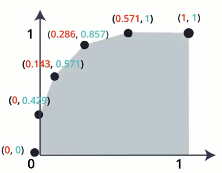
ROC curve through the points (0,0), (0,0.429), (0.143,0.571), (0.286,0.857), (0.571,1) and (1,1) with the area underneath shaded — The ROC curve of the 14 points: each dot is one boundary position, written (FPR, TPR). The shaded area is the AUC. *(From Dr. Albanna's slides; image from Udacity’s machine-learning course, Evaluation Metrics lesson (Luis Serrano).)*

Worked example — the area under the curve

Join the points with straight lines and add the trapezoids: 0.143 × (0.429 + 0.571)/2 + 0.143 × (0.571 + 0.857)/2 + 0.285 × (0.857 + 1)/2 + 0.429 × 1 = 0.072 + 0.102 + 0.265 + 0.429 = 0.87.

Reading the AUC

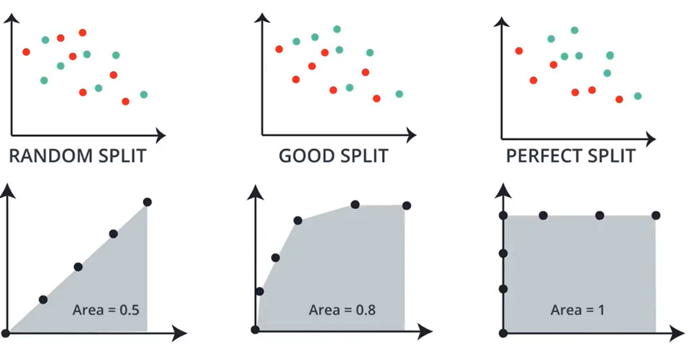
The AUC (Area Under the Curve) summarizes the whole curve in one number from 0 to 1. It equals the probability that the model gives a randomly chosen positive a higher score than a randomly chosen negative.

Random split with area 0.5, good split with area 0.8, perfect split with area 1 — A random split gives the diagonal (AUC = 0.5); a good split bulges toward the top-left corner (AUC ≈ 0.8); a perfect split hugs the corner (AUC = 1). *(From Dr. Albanna's slides; image from Udacity’s machine-learning course, Evaluation Metrics lesson (Luis Serrano).)*

AUC	Meaning
1.0	Perfect separation of the classes
0.9 – 1.0	Excellent
0.8 – 0.9	Good
0.7 – 0.8	Fair
0.5	No better than random guessing
< 0.5	Worse than random — the predictions are inverted

The coronary-disease model from Module 4

Left: ROC curve of the coronary-disease model with AUC 0.88 and the thresholds 0.3, 0.5 and 0.7 marked. Right: precision, recall and F1 as the threshold moves. — **Left:** the ROC curve of the age model (AUC = 0.88). The three thresholds from Module 4 are three points on the same curve. **Right:** raising the threshold raises precision and lowers recall; F1 peaks in between.

ROC curve of a classifier on the Default data, close to the top-left corner — A ROC curve for predicting credit-card default on 10,000 customers. The dotted diagonal is the “no information” classifier. *(Textbook T1: James, Witten, Hastie & Tibshirani, An Introduction to Statistical Learning with Applications in Python, Springer 2023, Figure 4.8.)*

ROC with k-fold cross-validation

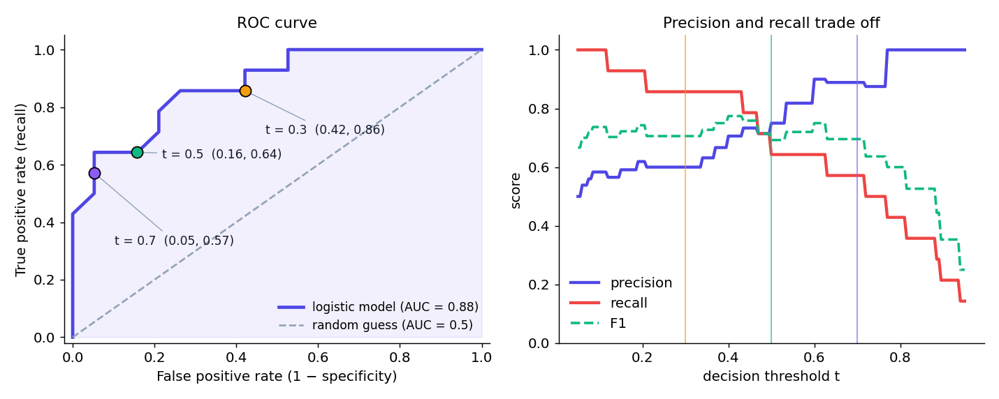
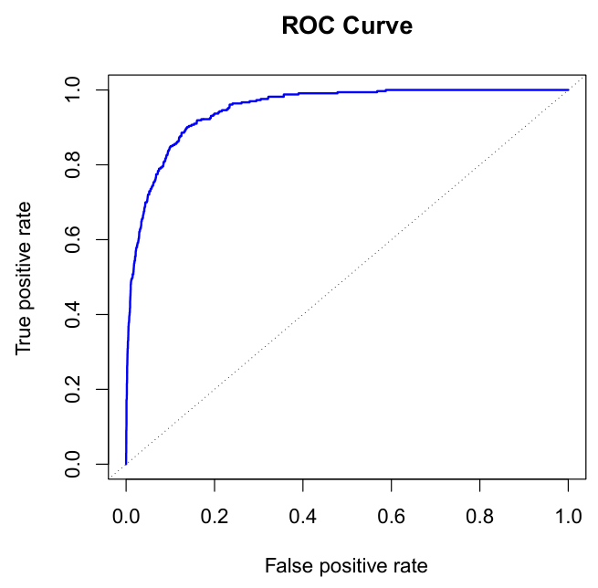
With k-fold cross-validation you get one ROC curve per fold. Plot them together with their mean curve and report the AUC as mean ± standard deviation — the spread shows how stable the model is.

10. Regression Metrics

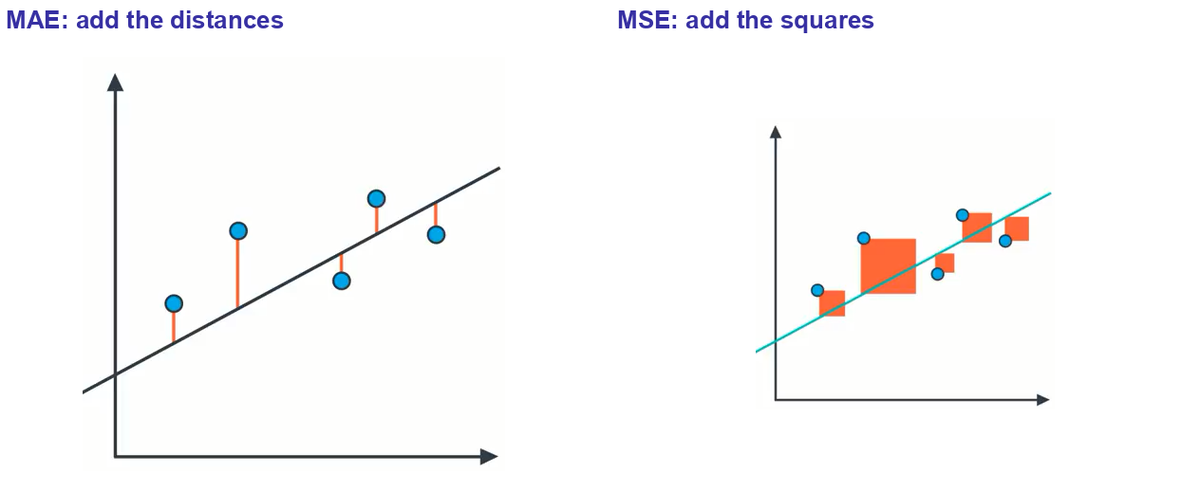
For regression there is no confusion matrix: we measure how far the predictions are from the true values. Draw a line through the points — but is it a good line or a bad one?

Left: vertical distances from the points to the line. Right: squares drawn on those distances. — **MAE** adds the absolute distances from the points to the line. **MSE** adds the areas of the squares on those distances. *(From Dr. Albanna's slides; image from Udacity’s machine-learning course, Evaluation Metrics lesson (Luis Serrano).)*

\[ \text{MAE} = \frac{1}{n}\sum_i |y_i - \hat y_i| \qquad \text{MSE} = \frac{1}{n}\sum_i (y_i - \hat y_i)^2 \qquad \text{RMSE} = \sqrt{\text{MSE}} \]

Metric	Units	Strength	Weakness
MAE	Same as y	Easy to read; robust to outliers	Not differentiable at 0, so awkward for gradient descent
MSE	y squared	Smooth and differentiable — the standard training loss	Large errors dominate; hard-to-read units
RMSE	Same as y	“Typical error” on the original scale	Still sensitive to outliers

R²: compare with the simplest model

What is the simplest possible model? A horizontal line at the mean of y. R² compares our model's error with that simple model's error:

The data, the squared errors of the mean line, and the much smaller squared errors of the regression line — (b) The mean line has large squared errors; (c) the regression line has much smaller ones. *(From Dr. Albanna's slides; image from Udacity’s machine-learning course, Evaluation Metrics lesson (Luis Serrano).)*

\[ R^2 = 1 - \frac{\text{MSE of the regression line}}{\text{MSE of the mean line}} = 1 - \frac{\sum(y_i - \hat y_i)^2}{\sum(y_i - \bar y)^2} \]

R2 = 1 minus the ratio of the two errors; a bad model has similar errors and R2 near 0, a good model has a much smaller error and R2 near 1 — If the two errors are similar, the line is no better than the mean and R² ≈ 0 (bad model). If the line's error is much smaller, R² ≈ 1 (good model). *(From Dr. Albanna's slides; image from Udacity’s machine-learning course, Evaluation Metrics lesson (Luis Serrano).)*

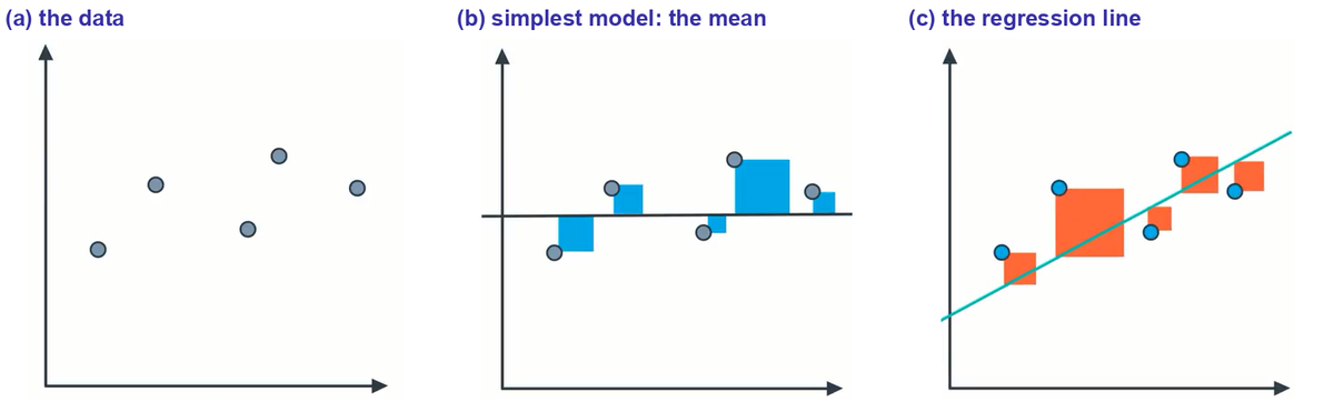
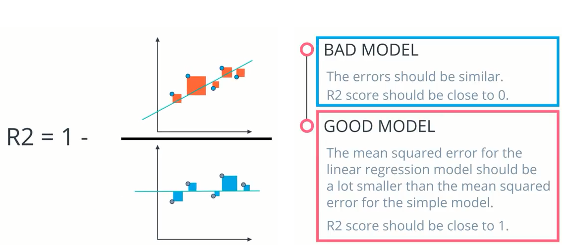
Adjusted R² = 1 − (1 − R²)(n − 1)/(n − k − 1) penalizes extra features (Module 3, Section 7).

Worked example

For the five points of Module 3 (from Statistics How To; ŷ = 9.2 + 0.8x): errors −2.6, 0.6, 3.8, 1.0, −2.8. MAE = 10.8 / 5 = 2.16; MSE = 30.4 / 5 = 6.08; RMSE = 2.47; R² = 1 − 30.4 / 36.8 = 0.17. The single error of 3.8 contributes 47% of the MSE but only 35% of the MAE — squaring magnifies large errors.

11. Choosing the Right Metric

Situation	Use	Why
Balanced classes, equal costs	Accuracy	Simple and fair when nothing is rare
Missing a positive is costly (disease, fraud)	Recall (sensitivity), F2	Count the misses
A false alarm is costly (spam, legal decisions)	Precision, F0.5	Count the false alarms
Imbalanced classes	F1, precision–recall curve, balanced accuracy	Accuracy is misleading
Comparing models across all thresholds	ROC curve, AUC	Threshold-independent
Several classes of unequal size	Macro-averaged F1	Small classes are not drowned out
Regression with outliers	MAE	Not dominated by a few large errors
Regression where large errors are dangerous	RMSE	Punishes large errors
How much of the variation is explained	R² / adjusted R²	Unit-free, compared with the mean model

Python Lab

Run this in Google Colab. It reproduces Example 1, the 4-class matrix from Exercise 4, and the regression example, then evaluates a classifier with stratified 10-fold cross-validation on five metrics.

import numpy as np
from sklearn.metrics import (confusion_matrix, accuracy_score, precision_score, recall_score, f1_score,
                             classification_report, mean_absolute_error, mean_squared_error, r2_score)
from sklearn.linear_model import LogisticRegression
from sklearn.model_selection import cross_val_score, StratifiedKFold
from sklearn.datasets import load_breast_cancer

# 1. Binary metrics: the cat example (TP=140, FN=30, FP=20, TN=10)
y_true = np.array([1] * 170 + [0] * 30)
y_pred = np.array([1] * 140 + [0] * 30 + [1] * 20 + [0] * 10)
print(confusion_matrix(y_true, y_pred, labels=[1, 0]))          # [[140 30] [20 10]]
print(f"accuracy={accuracy_score(y_true, y_pred):.3f}  precision={precision_score(y_true, y_pred):.3f}  "
      f"recall={recall_score(y_true, y_pred):.3f}  F1={f1_score(y_true, y_pred):.3f}  "
      f"specificity={recall_score(y_true, y_pred, pos_label=0):.3f}")  # specificity = recall of class 0

# 2. Multi-class: rebuild labels from a 4x4 matrix (rows = actual a..d, columns = predicted)
cm4 = np.array([[5, 23, 17, 17], [10, 540, 21, 14], [166, 96, 436, 110], [1, 2, 5, 87]])
y_t = np.repeat(np.repeat(np.arange(4), 4), cm4.ravel())
y_p = np.repeat(np.tile(np.arange(4), 4), cm4.ravel())
print(classification_report(y_t, y_p, target_names=list("abcd"), digits=3))  # per class + macro + weighted

# 3. Regression metrics: y_hat = 9.2 + 0.8x on five points
x = np.array([43, 44, 45, 46, 47]); y = np.array([41, 45, 49, 47, 44]); y_hat = 9.2 + 0.8 * x
print(f"MAE={mean_absolute_error(y, y_hat):.2f}  MSE={mean_squared_error(y, y_hat):.2f}  "
      f"RMSE={mean_squared_error(y, y_hat) ** 0.5:.2f}  R2={r2_score(y, y_hat):.3f}")   # 2.16 6.08 2.47 0.174

# 4. Stratified 10-fold cross-validation, five metrics, on a real dataset (569 tumours)
X, yb = load_breast_cancer(return_X_y=True)
model = LogisticRegression(max_iter=5000)
cv = StratifiedKFold(n_splits=10, shuffle=True, random_state=0)
for metric in ["accuracy", "precision", "recall", "f1", "roc_auc"]:
    s = cross_val_score(model, X, yb, cv=cv, scoring=metric)
    print(f"{metric:9s} {s.mean():.3f} ± {s.std():.3f}")
# accuracy 0.951, precision 0.954, recall 0.969, f1 0.961, roc_auc 0.994

Try it

In part 2, which class has the worst precision, and why? (Look at column a.) In part 4, add "balanced_accuracy" to the list of metrics.

The logistic-regression notebook from class also computes all these metrics: Logistic regression example (.ipynb)

Textbook Reading

From the course syllabus

T1 James et al. — ISLP, §2.2 Assessing Model Accuracy; §3.1.3 (RSE and R²); §4.4.2 (confusion matrix, sensitivity, specificity, ROC curve — Tables 4.4–4.7, Figure 4.8); §5.1 Cross-Validation.
T2 Murphy — Probabilistic Machine Learning, §5.1.3 ROC curves and §5.1.4 Precision–recall curves; §4.5.5 Cross-validation.

Both books are free to read online from their authors: statlearning.com (T1) and probml.github.io (T2).

Exercises

1

Pregnancy test

100 people: 40 are pregnant, of whom 30 are classified correctly; of the 60 who are not pregnant, 55 are classified correctly. Build the confusion matrix and compute accuracy, precision, recall and F1.

TP = 30, FN = 10, FP = 5, TN = 55. Accuracy = 85/100 = 0.85; precision = 30/35 = 0.857; recall = 30/40 = 0.75; F1 = 2(0.857)(0.75) / (0.857 + 0.75) = 0.80.

2

Read the rates

For the cat detector of Example 1, compute TPR, FNR, TNR and FPR, and check that each pair adds to 1.

TPR = 140/170 = 0.824, FNR = 30/170 = 0.176 (sum 1). TNR = 10/30 = 0.333, FPR = 20/30 = 0.667 (sum 1). A false-positive rate of 67% is the detector's real weakness.

3

F1 versus the average

Model A: precision 0.9, recall 0.1. Model B: precision 0.6, recall 0.5. Compute the arithmetic mean and F1 of each. Which model do the two measures prefer? Then compute F2 for model B.

Means: A = 0.50, B = 0.55. F1: A = 2(0.9)(0.1)/1.0 = 0.18; B = 2(0.6)(0.5)/1.1 = 0.545. The mean barely separates them, but F1 shows that A (which finds only 10% of the positives) is far worse. F2 for B = 5(0.6)(0.5) / (4(0.6) + 0.5) = 1.5 / 2.9 = 0.517.

4

Four classes

Rows are the actual class, columns the predicted class:

Actual \ Predicted	a	b	c	d	Total
a	5	23	17	17	62
b	10	540	21	14	585
c	166	96	436	110	808
d	1	2	5	87	95
Total	182	661	479	228	1550

Compute precision and recall for each class, the macro averages, and the accuracy.

Precision (diagonal / column total): a = 5/182 = 0.027, b = 540/661 = 0.817, c = 436/479 = 0.910, d = 87/228 = 0.382. Recall (diagonal / row total): a = 5/62 = 0.081, b = 540/585 = 0.923, c = 436/808 = 0.540, d = 87/95 = 0.916. Macro precision = 0.534, macro recall = 0.615. Accuracy = (5 + 540 + 436 + 87) / 1550 = 1068/1550 = 0.689. Class a is almost never recognized, and 166 class-c examples are wrongly called a — that is where to improve.

5

Build a ROC curve

Six test examples with scores and labels: 0.9 (+), 0.8 (+), 0.7 (−), 0.6 (+), 0.4 (−), 0.2 (−). Compute (FPR, TPR) at thresholds 0.75 and 0.5. Then compute the AUC as the fraction of (positive, negative) pairs in which the positive has the higher score.

Threshold 0.75: positives = {0.9, 0.8} → TP = 2, FP = 0 → (FPR, TPR) = (0, 0.667). Threshold 0.5: positives = {0.9, 0.8, 0.7, 0.6} → TP = 3, FP = 1 → (0.333, 1). AUC: 3 × 3 = 9 pairs; 0.9 and 0.8 beat all three negatives (6 pairs), 0.6 beats 0.4 and 0.2 (2 pairs) → AUC = 8/9 = 0.89.

6

Pick the metric

Which metric would you report for: (a) a fraud detector where 0.2% of transactions are fraud; (b) a house-price model where a few luxury homes have huge prices; (c) comparing two credit-scoring models before the bank has chosen a cut-off?

(a) Recall and precision (or F1 / the precision–recall curve) on the fraud class — accuracy would be 99.8% for a model that flags nothing. (b) MAE, so the few luxury homes do not dominate (report RMSE too if large errors are expensive). (c) ROC curve and AUC — they compare the models over all possible cut-offs.

Recap & Where Next

You now know

The confusion matrix (TP, FN, FP, TN) and the measures built on it: accuracy, error rate, precision, recall, specificity, F1, Fβ.
Accuracy is misleading on imbalanced data; precision counts false alarms, recall counts misses.
Multi-class metrics are computed per class and combined by macro or micro averaging.
The ROC curve plots TPR against FPR over all thresholds; the AUC summarizes it (0.5 random, 1 perfect).
Regression is measured by MAE, MSE, RMSE and R²; choose the metric that matches the cost of each mistake.

We now have the tools to compare classifiers. Module 6 introduces a classifier built from rules instead of equations: the decision tree.